Sound Power of Multisource Industrial Plants

A petrochemical complex, a quarry or a crushing plant is too large for the enveloping surface of ISO 3744 and too full of sources for any one of them to be measured alone. What its neighbours hear, at a few hundred metres, is the plant as a whole, and what a prediction model needs is one sound power level per octave band for that whole, placed at the centre of the plant area. ISO 8297 is the engineering method (grade 2 of ISO 2204) that measures it. A closed path, the measurement contour, is drawn round the plant on the plot plan; microphones stand on it at equal spacing, raised to a height that grows with the area the contour encloses and pointed horizontally at the plant; their octave-band levels are averaged; and four terms turn that average into the power. The method is for plants whose largest horizontal dimension lies between 16 m and about 320 m, which radiate roughly evenly in every horizontal direction, and whose result will be used at least 1.5 times that dimension from their centre (clauses 0.2 and 1.2).

The contour is any simply shaped closed path round the plant area $S_{\mathrm{p}}$, the area that holds every source. Three requirements fix how far out it runs and how densely it is sampled (9.1.1). The average measurement distance, the mean over the $N$ positions of the distance $d_i$ from each position to the nearest point of the plant perimeter,

shall exceed $0.05\sqrt{S_{\mathrm{p}}}$ or 5 m, whichever is the greater, and shall not exceed $0.5\sqrt{S_{\mathrm{p}}}$ or 35 m, whichever is the lesser. From any point of the contour the plant area shall be seen inside an aspect angle of at most 180°, which is to say the contour never dips into a notch of the plant. And adjacent positions shall be at most $2\bar{d}$ apart. The contour length $l$, the area it encloses $S_{\mathrm{m}}$ (the plant included) and the characteristic height of the plant, the mean height of the midpoints of its $n$ sources, $H=\frac{1}{n}{\sum }_k{h}_k$, are read off the plan to within ±5 % (9.2); where ten or more sources are lower than 2 m, NOTE 7 lets them be counted approximately and taken at 1 m. The microphone then stands at

at every position (9.3), its reference direction horizontal and at 90° to the contour, towards the plant (9.4).

plant_measurement_contour() takes the two polygons in metres and lays the positions along the contour from its first vertex. With no position_count it chooses the fewest that meet 9.1.1 c); give your own layout, and the positions a river or a building made you leave out (at most 10 %, 9.1.2.4), as position_count and omitted_positions.

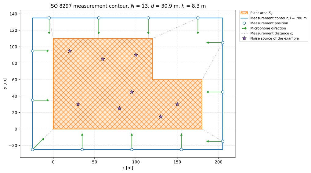
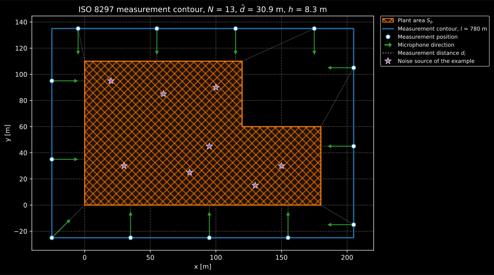
The contour of the example below. Thirteen positions are the fewest that keep 60 m between neighbours within $2\bar{d}=61.8$ m; the dotted lines are the $d_i$ whose mean is $\bar{d}$, and they run to the nearest point of the perimeter, which for the corner positions is a corner of the plant. The notch at the top right does not trouble 9.1.1 b): the contour stays outside the convex hull of the plant, so no point of it sees the plant over more than 149°.

import matplotlib.pyplot as plt
from phonometry import emission

plant = [[0, 0], [180, 0], [180, 60], [120, 60], [120, 110], [0, 110]]
contour_m = [[-25, -25], [205, -25], [205, 135], [-25, 135]]
source_heights_m = [3.0, 6.5, 12.0, 9.0, 4.0, 15.0, 7.5, 5.0]
H = emission.plant_characteristic_height_m(source_heights_m, low_source_count=14)
contour = emission.plant_measurement_contour(plant, contour_m, characteristic_height_m=H)
fig, ax = plt.subplots(figsize=(10.5, 5.8), layout="constrained")
contour.plot(ax=ax)
# The eight noise sources of the example in section 3, on the plan and in its legend.
source_xy = [(30, 30), (80, 25), (150, 30), (60, 85),
             (100, 90), (20, 95), (130, 15), (95, 45)]
(stars,) = ax.plot(*zip(*source_xy), "*", markersize=11, label="Noise source of the example")
legend = ax.get_legend()
labels = [text.get_text() for text in legend.get_texts()]
ax.legend([*legend.legend_handles, stars], [*labels, stars.get_label()], fontsize="small",
          loc="upper left", bbox_to_anchor=(1.02, 1.0), borderaxespad=0.0)
plt.show()

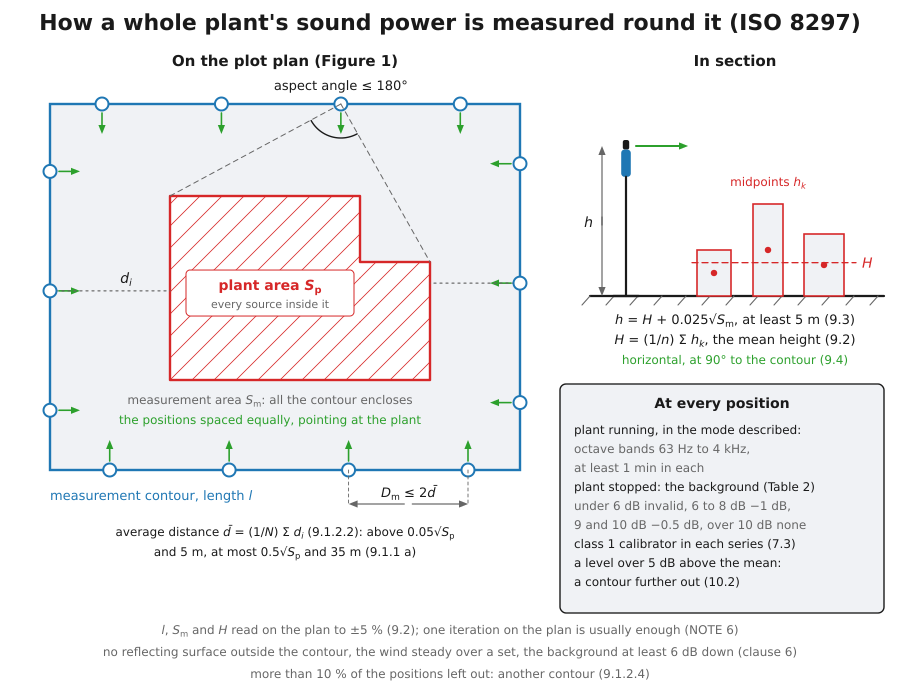
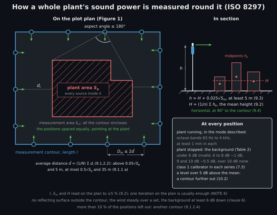
Draw a first contour on the plot plan, lay the positions on it and check 9.1.1 a) and b) there; if they fail, draw another (9.1.2.3; NOTE 6 expects one iteration to be enough). Measure $l$, $S_{\mathrm{m}}$ and $H$ on the plan, raise the microphones to the height of 9.3 (as high as possible above 5 m where it cannot be reached, and say so), and point them at the plant. Check the whole chain with a class 1 calibrator during each series. With the plant in the operating mode to be described, read the octave-band levels from 63 Hz to 4 kHz at every position (31.5 Hz and 8 kHz may be added), at least 1 min per band for a steady noise and with an integrating meter for anything else; where a sound level meter is used, a needle swinging less than 5 dB marks the noise as steady and the level is the mean of the maximum and the minimum (9.5.2); an integrating meter’s $L_{\mathrm{eq},T}$ is taken once it moves by no more than ±0.5 dB (9.5.3). With the plant stopped, read the background at the same positions. Keep the wind steady over a set, keep reflecting surfaces out from behind the microphones, and repeat the whole set for each operating mode (clauses 6 and 8).

Clause 10 is nine steps. The levels, each first corrected for the background by Table 2 (9.5.4, next section), are energy-averaged per band (step 1):

A level more than 5 dB above that average means the contour runs too close to one part of the plant; 10.2 asks for a contour further out, and where that is not practicable, replaces every such level by $\overline{L_p}+5$ dB and averages again into $\overline{L_p^{\ast }}$ (steps 2 and 3). plant_sound_power() does the latter with a SoundPowerWarning and records which levels it replaced in capped. Four terms then carry the average to the power (steps 4 to 8):

with $S_0=1$ m². Each has a plain reading. The area term is the measurement surface of ISO 3744: over a circular contour of radius $r$, $2S_{\mathrm{m}}=2\pi r^2$ is the hemisphere over it and $hl$ the band of wall of height $h$ round it, so a point source on the ground at the centre gives its own power back as the microphones come down to the ground. The proximity term takes back what the near sources add to the average; it has no factor 10, and NOTE 11 says it lies between −0.9 dB and −1.9 dB when 9.1 is met, which are $\lg (0.5/4)$ and $\lg (0.05/4)$, its values at the two ends of 9.1.1 a). The microphone term makes up for a directional microphone, whose 3 dB angle $\theta$ has to exceed 30° (7.1); it is 0 dB for an omnidirectional one. The air absorption term puts back what the air takes over half the root of the measurement area. The A-weighted level is the sum of the bands with the A-weighting $C_j$ (step 9), $L_{W\mathrm{A}}=10\lg {\sum }_{j}10^{0.1(L_{Wj}+C_j)}$ dB, with the octave-band values of ISO 3744:2010 Annex E that every sound power method of this library uses; a 31.5 Hz band, which Annex E does not weight, is left out of it.

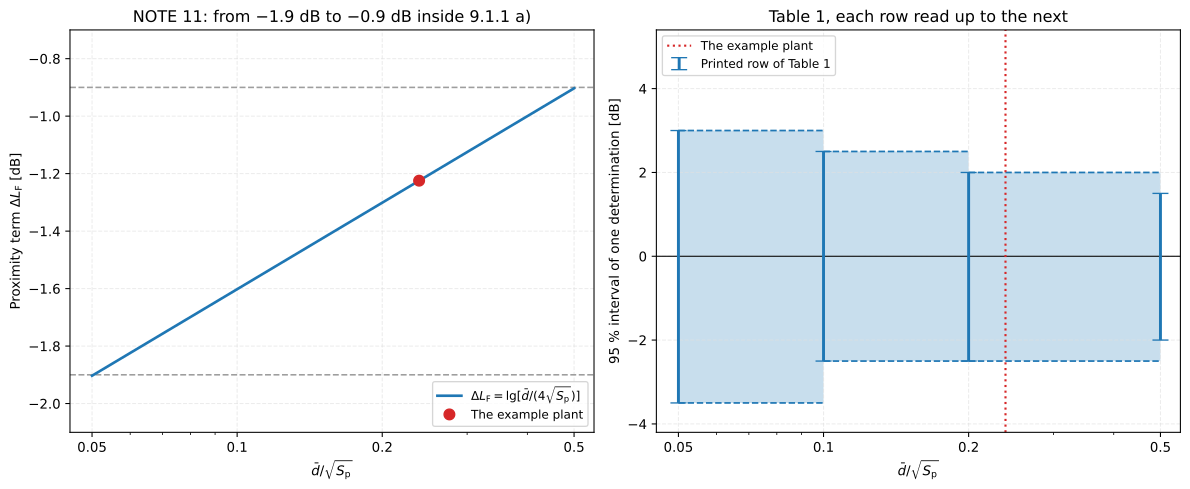
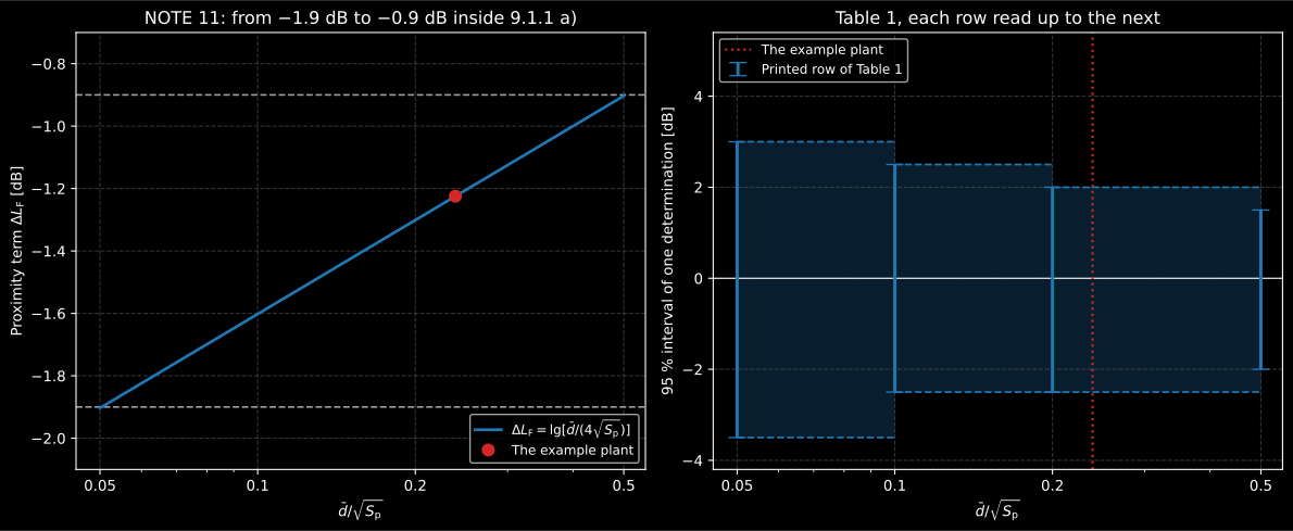
Everything the plan decides about the answer lives in one ratio, $\bar{d}/\sqrt{S_{\mathrm{p}}}$. On the left, the proximity term over the whole range 9.1.1 a) allows: one decibel from one end to the other, and never more negative than −1.9 dB. On the right, the uncertainty of Table 1 over the same range; the table prints four rows and says nothing between them, so a ratio between two rows takes the row below, the wider interval. The example plant sits at 0.24, in the $+2.0/-2.5$ dB row.

import matplotlib.pyplot as plt
import numpy as np
from phonometry import emission

ratio = contour.distance_ratio  # the example plant, from the contour above
ratios = np.geomspace(0.05, 0.5, 200)
fig, (axl, axr) = plt.subplots(1, 2, figsize=(12.5, 5.2))
axl.semilogx(ratios, np.log10(ratios / 4.0), label="dLF = lg(d / (4 sqrt(Sp)))")
axl.axhline(-0.9, linestyle="--")
axl.axhline(-1.9, linestyle="--")
axl.plot([ratio], [np.log10(ratio / 4.0)], "o", label="The example plant")
axl.set(xlabel="d / sqrt(Sp)", ylabel="Proximity term dLF [dB]")
axl.legend(loc="lower right")
rows = sorted(emission.PLANT_METHOD_UNCERTAINTY_DB)
lowers = [emission.PLANT_METHOD_UNCERTAINTY_DB[row][0] for row in rows]
uppers = [emission.PLANT_METHOD_UNCERTAINTY_DB[row][1] for row in rows]
# Each printed row is read up to the next: a shaded band with dashed edges.
for start, stop, lower, upper in zip(rows[:-1], rows[1:], lowers, uppers):
    axr.fill_between([start, stop], lower, upper, alpha=0.25)
    axr.hlines([lower, upper], start, stop, linestyles="--")
axr.errorbar(rows, [0.0] * len(rows), yerr=[[-v for v in lowers], uppers], fmt="none",
             capsize=6, label="Printed row of Table 1")
axr.axvline(ratio, linestyle=":", color="C3", label="The example plant")
axr.set(xscale="log", ylim=(-4.2, 5.4), xlabel="d / sqrt(Sp)", ylabel="95 % interval [dB]")
axr.legend(loc="upper left")
plt.show()

Where the plant can be stopped, the background is read at the same positions, and each level is corrected by the whole-decibel table of 9.5.4 before the average: 1 dB for a difference of 6, 7 or 8 dB, 0.5 dB for 9 or 10 dB, nothing above 10 dB, and “Measurement invalid” below 6 dB. A difference between two rows is rounded to the nearest whole decibel, a half going up; the two ends are taken as printed, so 5.9 dB is invalid and 10.2 dB is not corrected. plant_background_correction_db() reads the table on its own, and plant_sound_power() refuses a determination with a level less than 6 dB above its background, since the table has no correction to give it. Where the plant cannot be stopped, the levels go uncorrected, the report says so, and NOTE 1 warns that the uncertainty may then be larger than Table 1’s.

The example is an L-shaped crushing and screening plant, 180 m by 110 m, on the plan of the figure above, with a contour 25 m out. So that the answer can be checked, the thirteen microphones read what eight sources of known power would put there: each radiates over the ground as a hemisphere and loses $\alpha r$ to the air of Table 3. The background, read with the plant stopped, is 13 dB to 24 dB below.

import numpy as np
from phonometry import emission

plant = [[0, 0], [180, 0], [180, 60], [120, 60], [120, 110], [0, 110]]
contour_m = [[-25, -25], [205, -25], [205, 135], [-25, 135]]
# (x, y, height of the midpoint) in metres and LW from 63 Hz to 8 kHz, dB re 1 pW.
sources = [
    ((30, 30, 3.0), [108, 110, 109, 106, 103, 99, 93, 85]),  # primary crusher
    ((80, 25, 6.5), [104, 106, 106, 104, 101, 97, 91, 83]),  # secondary crusher
    ((150, 30, 12.0), [100, 103, 105, 104, 102, 99, 94, 87]),  # screen tower
    ((60, 85, 9.0), [98, 100, 101, 99, 96, 92, 86, 78]),  # conveyor transfer
    ((100, 90, 4.0), [101, 102, 100, 97, 94, 90, 84, 76]),  # generator set
    ((20, 95, 15.0), [97, 99, 100, 98, 95, 91, 85, 77]),  # stacker
    ((130, 15, 7.5), [99, 101, 101, 98, 95, 91, 85, 77]),  # compressor house
    ((95, 45, 5.0), [96, 98, 99, 97, 94, 90, 84, 76]),  # pumps
]
bands = np.array([63, 125, 250, 500, 1000, 2000, 4000, 8000], dtype=float)
alpha = emission.plant_air_absorption_db_per_m(bands)  # Table 3, 15 °C and 70 %


def levels_at(contour, sources):
    """What the microphones read: hemispherical spreading and alpha r."""
    h = contour.prescribed_microphone_height_m
    squares = 0.0
    for (x, y, z), lw in sources:
        dx = contour.positions_m[:, 0] - x
        dy = contour.positions_m[:, 1] - y
        r = np.sqrt(dx**2 + dy**2 + (h - z) ** 2)[:, None]
        level = np.array(lw) - 10 * np.log10(2 * np.pi * r**2) - alpha * r
        squares = squares + 10 ** (level / 10)
    return np.round(10 * np.log10(squares), 1)  # one row per position


# Fourteen motors and pumps lower than 2 m are counted by NOTE 7, at 1 m.
H = emission.plant_characteristic_height_m(
    [z for (_x, _y, z), _lw in sources], low_source_count=14
)
contour = emission.plant_measurement_contour(plant, contour_m, characteristic_height_m=H)
print(f"H = {H:.2f} m, N = {contour.positions_m.shape[0]}, "
      f"d = {contour.mean_distance_m:.1f} m, h = {contour.prescribed_microphone_height_m:.2f} m")
# H = 3.45 m, N = 13, d = 30.9 m, h = 8.25 m

levels = levels_at(contour, sources)
background = levels - np.array([14, 13, 15, 17, 19, 20, 22, 24])
result = contour.sound_power(levels, bands, background_levels_db=background)
print(np.round(result.mean_level_db, 1))
# [63.8 65.8 65.6 63.2 60.2 56.  49.1 39.9]
print(f"dLS = {result.area_term_db:.2f} dB, dLF = {result.near_field_term_db:.2f} dB")
# dLS = 49.03 dB, dLF = -1.22 dB
print(np.round(result.sound_power_level_db, 1))
# [111.6 113.6 113.5 111.2 108.5 104.8  99.4  92.1]
print(f"LWA = {result.a_weighted_sound_power_level_db:.1f} dB, Table 1: {result.uncertainty_db}")
# LWA = 113.5 dB, Table 1: (-2.5, 2.0)

The area term carries the average up by 49 dB, since the surface is some 80 000 m², and the proximity term takes 1.2 dB back. The air absorption term is nothing below 250 Hz and 4.4 dB at 8 kHz, where half the root of 36 800 m² of air is about 96 m at 0.046 dB/m. The eight sources radiate 113.0 dB(A) between them; ISO 8297 finds 113.5 dB(A), and 0.3 dB to 0.7 dB more in the bands up to 4 kHz, well inside the $+2.0/-2.5$ dB of Table 1.

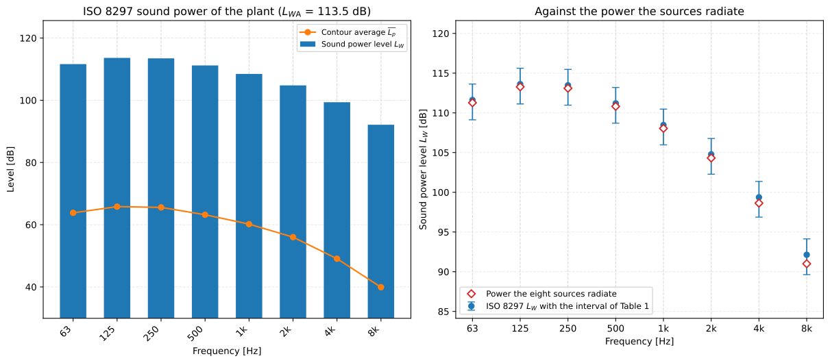
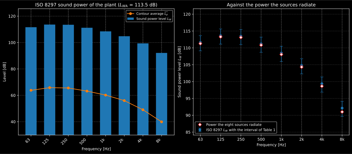
On the left, the figure result.plot() draws: the power per band beside the contour average it came from, the gap between them being the four terms. On the right, the same power against what the sources radiate, with the interval of Table 1. The method knows nothing of the sources; it reads thirteen levels, a plan and a height, and lands within half a decibel of the truth in the bands that carry $L_{W\mathrm{A}}$.

true_lw = 10 * np.log10(sum(10 ** (np.array(lw) / 10) for _p, lw in sources))
lower, upper = result.uncertainty_db
fig, (axl, axr) = plt.subplots(1, 2, figsize=(12.5, 5.4), layout="constrained")
result.plot(ax=axl)
x = np.arange(bands.size)
axr.errorbar(x, result.sound_power_level_db, yerr=[[-lower] * x.size, [upper] * x.size],
             fmt="o", capsize=4, label="ISO 8297 LW with the interval of Table 1")
axr.plot(x, true_lw, "D", markerfacecolor="white", label="Power the eight sources radiate")
axr.set_xticks(x)
axr.set_xticklabels([f"{f:g}" for f in bands])
axr.set(xlabel="Frequency [Hz]", ylabel="Sound power level LW [dB]")
axr.legend()
plt.show()

check_plant_measurement() holds the contour and the readings against the requirements of ISO 8297 that they decide, and returns one verdict. It cannot be used in an if by accident: its truth value raises, and the answer is passes.

check = emission.check_plant_measurement(
    contour, result, measurement_time_s=120.0, leq_range_db=0.6
)
print(check.passes, [r.key for r in check.failures], [r.key for r in check.deviations])
# True [] []
row = check.requirement("position_spacing")
print(f"{row.clause}: {row.value:.1f} m {row.comparison} {row.limit:.1f} m")
# 9.1.1 c): 60.0 m <= 61.8 m

The rows are clauses 1.2 (the largest dimension of the plant, 16 m to about 320 m), 9.1.1 a) to c), 9.1.2.4 (omitted positions), 9.3 (the microphone at least 5 m up), 7.1 (a directional microphone’s 3 dB angle above 30°), 6 b) (the background at least 6 dB below), 9.5.1 a) (the seven bands from 63 Hz to 4 kHz), 9.5.1 (a minute per position) and, given leq_range_db, 9.5.3 (an integrated reading that moves by no more than ±0.5 dB, a range of 1 dB). Four more are advisory: the standard lets them go unmet provided the report says so, so they are listed in deviations and do not decide passes. The first is the height of 9.3 itself, which is a height to stand at rather than a lower bound: the row holds when the microphones stand at it to within the ±5 % to which 9.2 reads $H$ and $S_{\mathrm{m}}$ off the plan, and a microphone lower (as high as possible, where the height cannot be reached) or higher is a deviation to report. The others are the background “preferably more than 10 dB” below, a level more than 5 dB above the average (10.2), and the “approximately 320 m” of 1.2.

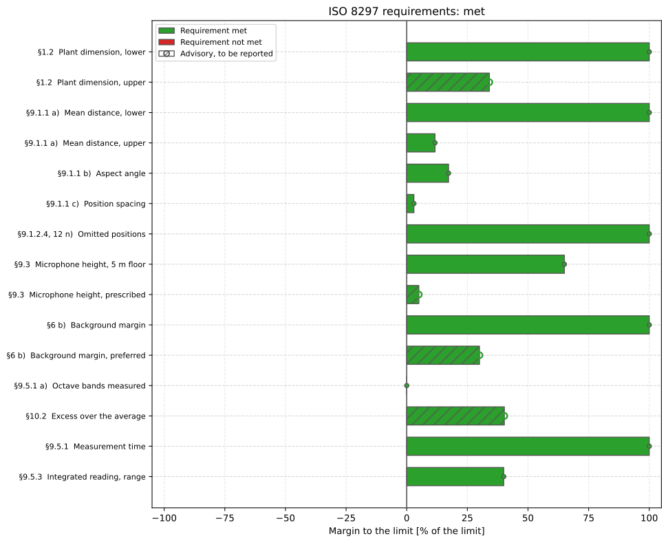
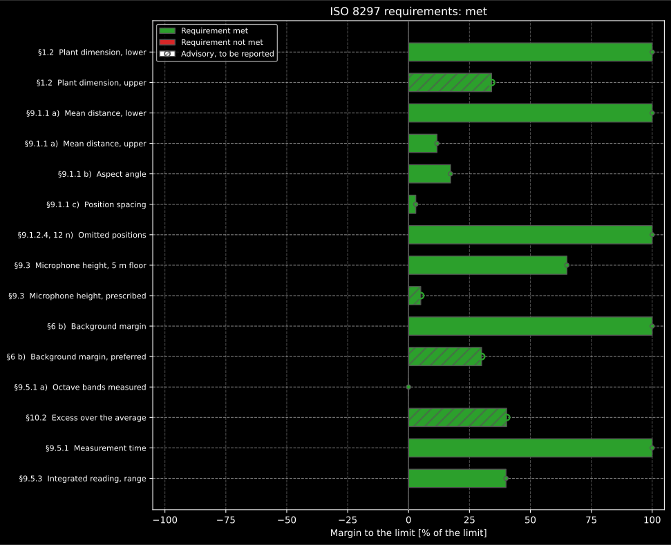
The verdict on the example, drawn by check.plot(). The tightest margin is the spacing: thirteen positions put 60 m between neighbours against the 61.8 m that $2\bar{d}$ allows, which is why twelve would not do. The microphones stand at the prescribed height, so that row keeps the whole ±5 % the plan allows it. One row sits at exactly zero, the octave bands: the seven required, 63 Hz to 4 kHz, are all among the eight measured, and a count of them cannot exceed seven.

fig, ax = plt.subplots(figsize=(10.0, 8.1), layout="constrained")
check.plot(ax=ax)
plt.show()

Table 3 prints $\alpha$ per octave band at 15 °C and 70 %, “taken from ISO 3891”, and asks for the values at the temperature and humidity of the measurement when the weather differs markedly. plant_air_absorption_db_per_m() returns the table as printed when no weather is given. Given a temperature and a relative humidity, it evaluates the attenuation coefficient of ISO 3891 Annex A, the SAE ARP 866A formula, at the one-third-octave band centred on each octave, through the same implementation the NPD curves for the air at the airport use; ISO 3891 gives no evaluation frequency below 50 Hz, so the 31.5 Hz band keeps the 0 of Table 3. Since the formula does not return Table 3 at 15 °C and 70 % (see the figure), passing those very conditions is not the same as passing none: at 8 kHz it gives $0.5\times 0.0148\sqrt{S_{\mathrm{m}}}\approx 0.0074\sqrt{S_{\mathrm{m}}}$ dB more in the power, 1.4 dB over the 36 800 m² of the example. Pass the weather when it differs markedly from 15 °C and 70 %, which is when Table 3 asks for it; the standard puts no number on “markedly”.

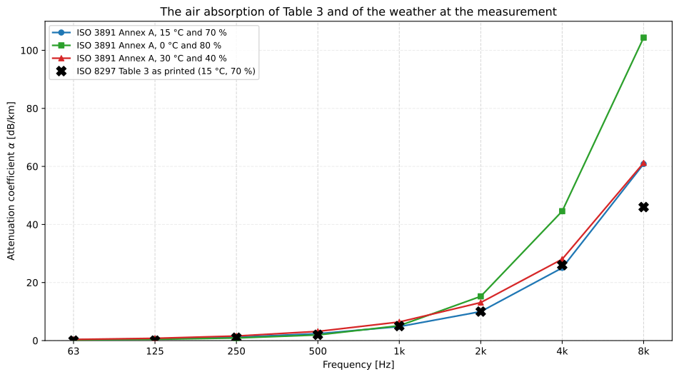
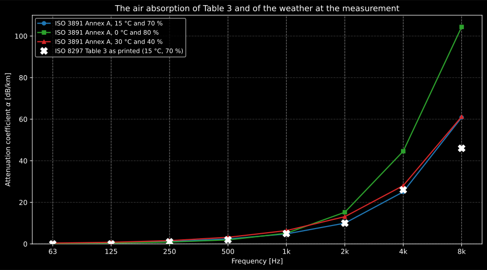
Table 3 and the formula it was taken from. They meet at 63 Hz and from 250 Hz to 2 kHz to the printed digit, and not in three rows: 125 Hz, where the formula gives 0.000 59 dB/m and the table 0; 4 kHz, 0.025 05 against 0.026; and 8 kHz, 0.061 against 0.046. ISO 3891 Table 9 itself prints 0.1, 2.5 and 6.1 dB/100 m in those bands at 15 °C and 70 %, and no single weather makes the formula reproduce Table 3 in every row. ISO 8297 does not say how it drew its octave values from the one-third-octave data of ISO 3891, so the table is used as printed and the difference is stated here rather than corrected.

x = np.arange(bands.size)
fig, ax = plt.subplots(figsize=(10.0, 5.6))
for temperature_c, humidity in ((15.0, 70.0), (0.0, 80.0), (30.0, 40.0)):
    coefficient = emission.plant_air_absorption_db_per_m(
        bands, temperature_c=temperature_c, relative_humidity_percent=humidity
    )
    ax.plot(x, 1000 * coefficient, marker="o",
            label=f"ISO 3891 Annex A, {temperature_c:g} °C and {humidity:g} %")
ax.plot(x, 1000 * emission.plant_air_absorption_db_per_m(bands), "X",
        label="ISO 8297 Table 3 as printed (15 °C, 70 %)")
ax.set_xticks(x)
ax.set_xticklabels([f"{f:g}" for f in bands])
ax.set(xlabel="Frequency [Hz]", ylabel="Attenuation coefficient [dB/km]")
ax.legend()
plt.show()

For the example plant, measured on a warm dry afternoon, the weather moves only the air term: against Table 3 the power at 8 kHz rises by 2.4 dB and $L_{W\mathrm{A}}$ by 0.1 dB. Of those 2.4 dB, 1.4 dB is the step from Table 3 to the formula, which 15 °C and 70 % already take; the warm dry air itself adds 1.0 dB.

warm = contour.sound_power(levels, bands, background_levels_db=background,
                           temperature_c=25.0, relative_humidity_percent=40.0)
print(np.round(warm.sound_power_level_db - result.sound_power_level_db, 2))
# [0.03 0.07 0.04 0.08 0.08 0.19 0.34 2.4 ]
reference = contour.sound_power(levels, bands, background_levels_db=background,
                                temperature_c=15.0, relative_humidity_percent=70.0)
print(np.round(warm.sound_power_level_db - reference.sound_power_level_db, 2))
# [0.01 0.01 0.02 0.05 0.1  0.19 0.43 0.97]
print(f"LWA = {warm.a_weighted_sound_power_level_db:.1f} dB")
# LWA = 113.6 dB

The method also serves to find what particular parts of an industrial area contribute and to compare installations (0.2 b and c). Each part is measured round its own contour, and partial_plant_contributions() puts them together: the parts radiate incoherently, so the whole is the energy sum of their powers band by band, and each part’s contribution is its level less that sum. NOTE 2 is the caveat that goes with it: the power of a plant measured round one contour may differ from the sum of the powers of its sources, so a sum of parts is not the same determination as the whole area measured at once. Here the crushing plant shares its industrial area with an asphalt mixing plant 120 m to the east.

# An asphalt mixing plant in the same industrial area, 60 m by 40 m, with its
# own contour 15 m out and its own three sources.
asphalt_plant = [[300, 20], [360, 20], [360, 60], [300, 60]]
asphalt_sources = [
    ((315, 40, 4.0), [106, 105, 103, 100, 97, 93, 87, 79]),  # dryer drum and burner
    ((340, 30, 8.0), [100, 102, 101, 98, 95, 91, 85, 77]),  # exhaust fan and bag house
    ((350, 52, 12.0), [95, 97, 97, 95, 92, 88, 82, 74]),  # mixing tower
]
asphalt = emission.plant_measurement_contour(
    asphalt_plant,
    [[285, 5], [375, 5], [375, 75], [285, 75]],
    characteristic_height_m=emission.plant_characteristic_height_m([4.0, 8.0, 12.0]),
)
asphalt_result = asphalt.sound_power(levels_at(asphalt, asphalt_sources), bands)
print(f"LWA = {asphalt_result.a_weighted_sound_power_level_db:.1f} dB")
# LWA = 105.4 dB

area = emission.partial_plant_contributions(
    [result, asphalt_result], names=["Crushing and screening", "Asphalt mixing"]
)
print(f"LWA of the area = {area.a_weighted_total_db:.1f} dB")
# LWA of the area = 114.1 dB
print(np.round(area.a_weighted_contribution_db, 1))
# [-0.6 -8.7]

Sources raised well above the characteristic height of the plant, which screening or their own directivity kept out of the contour’s reading, are determined by the standard that fits them (ISO 3744 or ISO 3746, for example) and reported beside the plant (clause 11, and item m) of clause 12); they are not added into its $L_W$.

The crushing plant is 0.6 dB below the total of the area and the asphalt plant 8.7 dB below it: noise control at the crusher is where the decibels are. area.plot() draws each part’s $L_W$ and the total band by band.

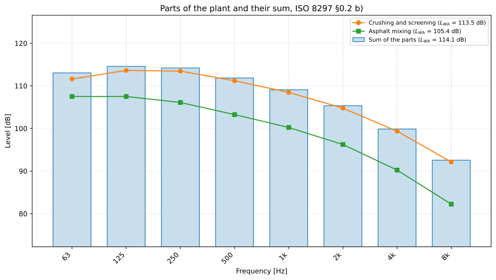
The two plants of the area and their sum, drawn by area.plot(). The crushing plant sits within 1.4 dB of the sum in every band, so it sets the power of the area; the asphalt plant adds 0.6 dB to the A-weighted total.

fig, ax = plt.subplots(figsize=(10.0, 5.6), layout="constrained")
area.plot(ax=ax)
plt.show()

Table 1 states the uncertainty inherent in the method as a 95 % confidence interval for one determination, and makes it depend on one thing, $\bar{d}/\sqrt{S_{\mathrm{p}}}$: $+3.0/-3.5$ dB at 0.05, $\pm 2.5$ dB at 0.1, $+2.0/-2.5$ dB at 0.2 and $+1.5/-2.0$ dB at 0.5. The interval is not symmetric, and it narrows as the contour moves out, because it comes from the spread of the levels round the contour that an uneven distribution of sources causes; a contour further out sees the plant more evenly. It does not include a change of the emission over time, and where the background could not be corrected NOTE 1 says it may be larger. plant_method_uncertainty_db() reads the table, and every result carries it as uncertainty_db.

• Covered

  The ISO 8297:1994 engineering method, every step that turns the plan and the readings into numbers: the contour and its positions, directions and distances from two polygons (plant_measurement_contour), the characteristic height with NOTE 7 (plant_characteristic_height_m), the microphone height of 9.3, the window of 9.1.1 a) and the largest aspect angle of 9.1.1 b) on the contour; the background correction of Table 2, the steady reading of 9.5.2 and the steadiness of an integrated reading of 9.5.3; the nine steps of clause 10 (plant_sound_power) with the air absorption of Table 3 or of ISO 3891 Annex A for the weather at the measurement; the uncertainty of Table 1; the verdict on 1.2, 6 b), 7.1, 9.1, 9.3, 9.5.1, 9.5.3 and 10.2 (check_plant_measurement); and the parts of a plant put together (partial_plant_contributions). The standard prints no worked example, so the conformance report anchors the chain in its three tables, the bound of NOTE 11, ISO 3891 Table 9 and closed forms.

• Not covered

  Left to the measurement team by choice, although some of it carries a printed number: the accuracy the plan is read to (±5 %, and ±30 % for $\bar{d}/\sqrt{S_{\mathrm{p}}}$), the calibration intervals of 7.3, the reflecting surfaces and the wind of clause 6 a) and c), and the report of clause 12. The sound power of sources raised above the plant (clause 11) belongs to other standards and is not summed into the plant’s. Table 3 is used as printed where it departs from the ISO 3891 coefficient it cites.

References

Section titled “References”- International Organization for Standardization. (1978). Acoustics — Procedure for describing aircraft noise heard on the ground (ISO 3891:1978). Annex A, the SAE ARP 866A attenuation coefficient that ISO 8297 Table 3 was taken from and that this guide evaluates for the weather at the measurement. Withdrawn.
- International Organization for Standardization. (1994). Acoustics — Determination of sound power levels of multisource industrial plants for evaluation of sound pressure levels in the environment — Engineering method (ISO 8297:1994). The contour of 9.1, the plant dimensions of 9.2, the microphone height and direction of 9.3 and 9.4, the background correction of Table 2, the nine steps of clause 10 with the air absorption of Table 3, and the uncertainty of Table 1 that this guide implements; read in the identical British adoption BS ISO 8297:1994.