NPD data for the air at the airport

The noise-power-distance (NPD) curves of the ANP database were measured in whatever air the certification tests happened to have, and then normalised to one atmosphere so that curves from different aircraft can be compared. That atmosphere is SAE AIR-1845: the arithmetic mean of the attenuation rates recorded in European and US certification tests. It is not a temperature and a humidity; no real air absorbs exactly like it in every band, and ECAC Doc 29 calls it a purely notional atmosphere.

An airport is not notional. A cold, humid coastal field absorbs less at high frequency than the average test day, so its aircraft are louder far from the runway than the database says; a hot, dry one can absorb more. ECAC Doc 29 Vol. 2 Appendix D recalculates the NPD curves for the air of a study, and this guide runs it: from the AIR-1845 rates, through the spectral class that each NPD carries, to revised curves that feed the event levels and contours of Airport Noise (ECAC Doc 29) and The ANP fleet database.

Table D-1 is the whole of it: one attenuation rate per one-third-octave band, in decibels per 100 m, from 50 Hz to 10 kHz.

from phonometry import aircraft

rates = aircraft.SAE_AIR1845_ATTENUATION_DB_PER_100M
print(rates[1000.0], rates[10000.0])   # 0.59 9.836 dB/100 m

The table is read-only, like every table the library publishes. Appendix D suggests computing the rates of the study atmosphere and comparing them with these before deciding whether an adjustment is needed at all; the increment of section 3 is that comparison carried through to the level.

An NPD table gives A-weighted levels, and absorption acts band by band, so the recalculation needs a spectrum. Every ANP aircraft is assigned two spectral classes, one for approach and one for departure: the average unweighted spectrum of a family of aircraft at the time of the maximum level, at 1000 ft, normalised to the same AIR-1845 rates and, for historical reasons, to 70 dB in the 1 kHz band (Doc 29 Vol. 2, G4.3). The database ships 41 of them in Spectral_classes.csv, and phonometry now reads it.

from phonometry import aircraft

db = aircraft.load_anp_database()
ac = db.aircraft("747100")
print(ac.departure_spectral_class_id, ac.approach_spectral_class_id)   # 107 209
spectrum = ac.spectral_class("D")
print(spectrum.description, spectrum.levels_db[13])   # 4-Engine.Tfan 70.0 dB at 1 kHz
print(db.spectral_class(103).description)             # 2-Engine.HighByPass.Tfan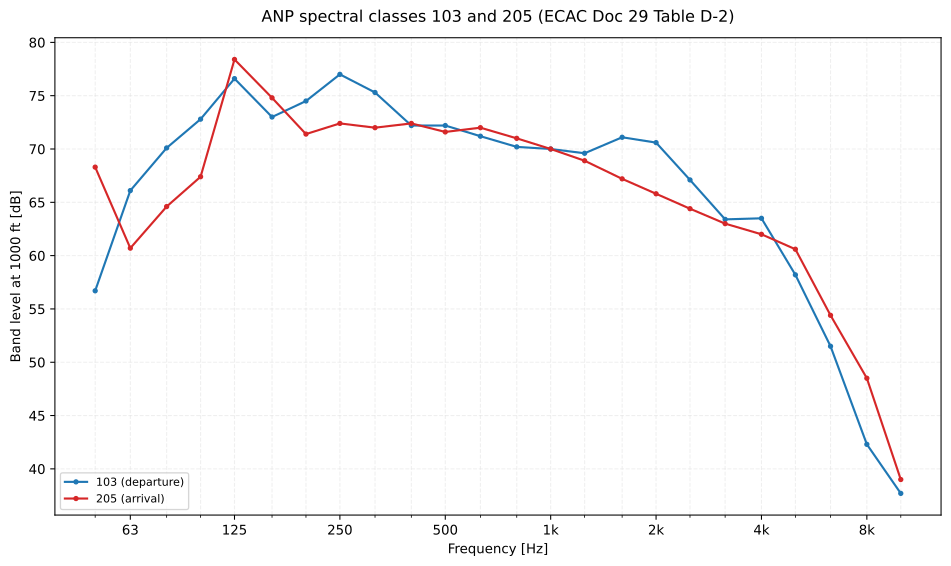

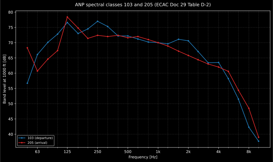
The two spectral classes of the Appendix D example, as the database ships them and as Table D-2 prints them. Both pass through 70 dB at 1 kHz by construction; the approach class keeps more energy above 5 kHz, where absorption is strongest.

import matplotlib.pyplot as plt
from phonometry import aircraft

db = aircraft.load_anp_database()
fig, ax = plt.subplots(figsize=(10, 6))
db.spectral_class(103).plot(ax=ax)
db.spectral_class(205).plot(ax=ax, color="tab:red")
ax.set_title("ANP spectral classes 103 and 205 (ECAC Doc 29 Table D-2)")
plt.show()

With the spectral class $L_{n,\mathrm{ref}}(d_{\mathrm{ref}})$ at $d_{\mathrm{ref}}$ = 1000 ft = 304.8 m and the AIR-1845 rate ${\alpha }_{n,\mathrm{ref}}$ of band $n$, Appendix D first adds the reference attenuation back (Eq. D-1), then takes the spectrum to each NPD distance $d_i$ twice, once in each atmosphere (Eqs. D-2 and D-3), and finally A-weights and sums both (Eq. D-4). The rates are the decibels lost over 100 m of path, as Table D-1 prints them, and the distances are in metres, so every attenuation term carries the conversion $d/(100\mathrm{m})$:

Doc 29 prints the same equations with the rates in dB/m. At 1 kHz the rate of 0.59 dB/100 m puts back $0.59\times 304.8/100$ = 1.80 dB over $d_{\mathrm{ref}}$, the 1.798 dB of Table D-3a, and the 70.0 dB of the class becomes the 71.8 dB that Table D-2 prints at the source. ${\delta }_n(d_i)$ is the rate of the specified air in the same unit, which under ARP 5534 also depends on the path length and the pressure, so ${\delta }_n(d_i)d_i/(100\mathrm{m})$ is its band attenuation over the path. $A_n$ is the A-weighting as an attenuation: the nominal values of IEC 61672-1, to 0.1 dB, which Doc 29 names without printing and which are the ones that reproduce its tables. The increment $\Delta L$ is added to the NPD level at the same distance, for every power setting and for $L_{\max }$ and $L_E$ alike: the change of air is taken to alter the spectrum, not the shape of the level time history. Because $\Delta L$ is a difference of two sums over the same spectrum, the 70 dB normalisation of the class drops out of it.

import numpy as np
from phonometry import aircraft

db = aircraft.load_anp_database()
increment = aircraft.npd_atmosphere_increment(
    db.spectral_class(103), temperature_c=10.0, relative_humidity_percent=80.0
)
print(round(increment.reference_attenuation_db[13, 3], 3))   # 1.798 dB, 1 kHz over 1000 ft
print(round(increment.source_spectrum_db[13], 1))            # 71.8 dB, Eq. D-1
print(np.round(increment.reference_levels_dba, 1))   # 97.0 90.3 ... 35.3 dBA
print(np.round(increment.increment_db, 1))
# [0.1 0.3 0.4 0.7 1.2 1.8 2.1 2.4 2.9 3.6] dB, 200 ft to 25000 ft

Those are the numbers of Table D-4. At 10 °C and 80 % the air absorbs less than the AIR-1845 average in the bands that matter, so the NPD levels rise, by a tenth of a decibel at 200 ft and by 3.6 dB at 25000 ft. The temperature and the humidity are keyword-only and have no default: the AIR-1845 atmosphere is not a pair of them, so there is no reference value to fall back to.

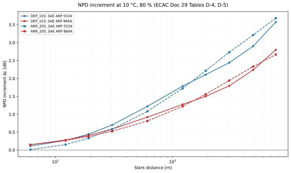
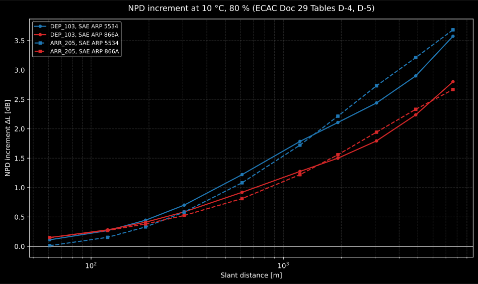
The increment of Tables D-4 and D-5 for both spectral classes and both absorption routes. The two routes agree within about 0.3 dB up to 2000 ft (610 m) and part beyond it, by up to a decibel at 25000 ft.

import matplotlib.pyplot as plt
from phonometry import aircraft

db = aircraft.load_anp_database()
fig, ax = plt.subplots(figsize=(10, 6))
for class_id, operation, style, marker in ((103, "DEP", "-", "o"),
                                           (205, "ARR", "--", "s")):
    for route, name, color in (("arp5534", "SAE ARP 5534", "tab:blue"),
                               ("arp866a", "SAE ARP 866A", "tab:red")):
        aircraft.npd_atmosphere_increment(
            db.spectral_class(class_id), absorption=route,
            temperature_c=10.0, relative_humidity_percent=80.0,
        ).plot(ax=ax, color=color, ls=style, marker=marker,
               label=f"{operation}_{class_id}, {name}")
ax.set_title("NPD increment at 10 °C, 80 % (ECAC Doc 29 Tables D-4, D-5)")
plt.show()

Appendix D offers two ways to compute ${\delta }_n(d_i)$, and absorption= picks one.

SAE ARP 5534 ("arp5534", the default and the route Doc 29 recommends) evaluates the pure-tone coefficient at the exact mid-band frequency and maps the pure-tone attenuation over the path to a band attenuation with the SAE Method, so the band attenuation depends on the path length and on the pressure. It is sae_band_attenuation of the certification guide. Its pure-tone coefficient is the one of ISO 9613-1 with the saturation vapour pressure that ARP 5534 prints in its Eqs. 5-6, the longer form of ANSI S1.26; with the shorter ISO 9613-1 form 57 of the 240 cells of Table D-3c come out up to 0.036 dB off, and with Eqs. 5-6 all 240 agree to the last printed digit.

SAE ARP 866A ("arp866a", kept by Doc 29 for transition) is an attenuation rate per band that depends on temperature and humidity only. SAE ARP 866A is not reachable as a document of its own; its formula is given in ISO 3891:1978 Annex A, which is where phonometry implements it from, as arp866a_attenuation:

import numpy as np
from phonometry import aircraft

absorption = aircraft.arp866a_attenuation(
    [1000.0, 10000.0], temperature_c=10.0, relative_humidity_percent=80.0
)
print(absorption.evaluation_frequencies_hz)             # [1000. 9000.] Hz
print(np.round(absorption.coefficient_db_per_100m, 3))  # [0.439 9.774] dB/100 m

for reading in ("quadratic", "linear"):
    band = aircraft.arp866a_attenuation(
        [4000.0], temperature_c=10.0, relative_humidity_percent=80.0,
        eta_interpolation=reading,
    )
    print(reading, np.round(band.path_attenuation_db(7620.0), 1))
# quadratic [203.1], linear [204.4] dB over 25000 ft; Table D-3b prints 204.355

Two details of Annex A decide those numbers. Above 4 kHz the formula is evaluated at the lower edge of the band, not at its centre, because the steep fall of an aircraft spectrum puts most of a high band’s energy at its lower end; Table 2 prints those frequencies rounded, 4500, 5600, 7100 and 9000 Hz, and the 10 kHz band above is evaluated at 9 kHz. And the factor $\eta (\delta )$ comes from Table 1, whose note says “a form of quadratic interpolation shall be used” without saying which, and the two documents that print this attenuation read it differently. ISO 3891’s own Table 10 (80 %, -10 °C to 40 °C) is reproduced in all its 264 cells by the parabola through three neighbouring entries of Table 1, which is the default of arp866a_attenuation; linear interpolation misses 11 of them. Doc 29 Table D-3b, and through it Tables D-5 and D-6c, is reproduced by linear interpolation, which the quadratic misses by up to 1.2 dB at 25000 ft, so the Appendix D route reads $\eta$ linearly. The two part only where $\delta$ falls in the curved part of Table 1, below 6.50 (from there on Table 1 prints 0.200 and both readings hold it), and the increments they give differ by a few thousandths of a decibel.

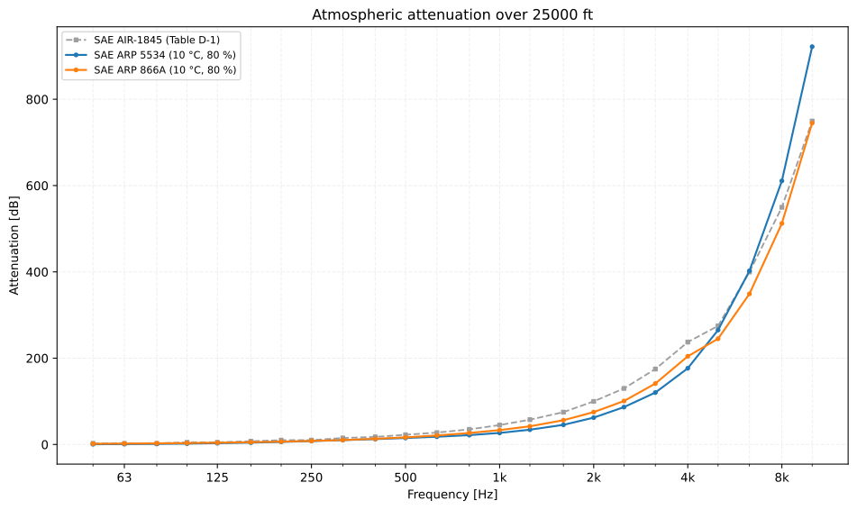
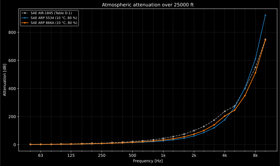
The attenuation of Tables D-3a to D-3c at the longest NPD distance. Where a curve lies below the dashed AIR-1845 one the specified air absorbs less than the average test day, and the NPD level at that distance goes up. Over 25000 ft the bands from 1 kHz up carry at most about 1 % of the A-weighted level in any of the three atmospheres, and the bands from 125 Hz to 500 Hz about nine tenths of it, so the increment there is decided from 125 Hz to 500 Hz, where ARP 5534 absorbs less than ARP 866A and both less than AIR-1845.

import matplotlib.pyplot as plt
from phonometry import aircraft

spectrum = aircraft.load_anp_database().spectral_class(103)
fig, ax = plt.subplots(figsize=(10, 6))
for route, reference in (("arp5534", True), ("arp866a", False)):
    aircraft.npd_atmosphere_increment(
        spectrum, absorption=route,
        temperature_c=10.0, relative_humidity_percent=80.0,
    ).plot_attenuation(ax=ax, distance_m=25000 * 0.3048, reference=reference)
plt.show()

revise_npd_curves adds the increment to every power setting of an AnpNpdCurves, and AnpDatabase.revised_npd_curves does it with the aircraft’s own spectral class. The revised curves are an ordinary AnpNpdCurves, so level, plot and the Doc 29 functions read them like the database’s own.

from phonometry import aircraft

db = aircraft.load_anp_database()
revised = db.revised_npd_curves(
    "747100", "D", "SEL", temperature_c=30.0, relative_humidity_percent=30.0
)
before = float(revised.original.levels[0, -1])
after = float(revised.revised.levels[0, -1])
print(round(before, 1), round(after, 1))   # 63.4 62.9 dB at 25000 ft, 20000 lb
revised.plot()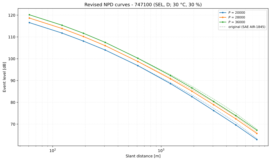

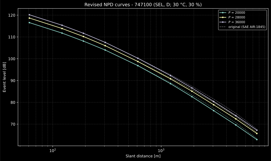
A hot, dry day on a four-engined departure. The increment is negative: this air absorbs more than the AIR-1845 average in the bands that carry the A-weighted level at long range, so beyond about 1 km the revised curves fall below the database ones, by up to 1.1 dB at 3 km, while close to the aircraft the two are the same curve.

import matplotlib.pyplot as plt
from phonometry import aircraft

revised = aircraft.load_anp_database().revised_npd_curves(
    "747100", "D", "SEL", temperature_c=30.0, relative_humidity_percent=30.0
)
fig, ax = plt.subplots(figsize=(10, 6))
revised.plot(ax=ax)
plt.show()

For a whole event or a contour there is no need to revise anything by hand. The event and contour wiring of the database takes the humidity, recalculates both the SEL and the LAmax tables with the aircraft’s spectral class, and uses the same temperature and pressure it already reads for the impedance adjustment: there is one air at the field, and the humidity completes it.

from phonometry import aircraft

db = aircraft.load_anp_database()
receiver = [6000.0, 0.0, 0.0]
reference = db.event_level("747100", receiver, "D", temperature_c=10.0)
humid = db.event_level(
    "747100", receiver, "D", temperature_c=10.0, relative_humidity_percent=80.0
)
print(round(reference.level, 1), round(humid.level, 1))   # 97.8 99.1 dB SEL

Leave relative_humidity_percent unset and nothing changes: the curves stay in the AIR-1845 atmosphere, as they always have. With an Aerodrome, the temperature and the field pressure come from it.

Appendix D closes with a worked example that prints every intermediate table, and each one is a row of the conformance report: the source spectra of Table D-2, the three attenuation tables D-3a to D-3c, the A-weighted levels and increments of Tables D-4 and D-5, and the revised JETW data of Tables D-6b and D-6c, cell by cell at the precision they are printed to. All of them agree to the last digit but two. In Table D-3b, 32 of the 240 cells, the longest paths at the highest frequencies, are printed about 6 parts per million below the ISO 3891 formula, at most 0.0045 dB of 745 dB; the row allows for it and says so. And the last row of Table D-6c is printed as a copy of the last row of Table D-6b, which is in the errata register together with a sentence of the appendix that pairs Tables D-3b and D-3c with each other’s method.

ISO 3891 is checked on its own terms as well: its Table 10 is a row of the report, all 264 cells from -10 °C to 40 °C to the printed digit. Its Table 9, at 70 %, is not, and the formula misses 15 of its cells by one printed unit. In seven of them the humidity drops out of the formula, so the two tables have to print the same value, and Table 9 prints one unit more than Table 10; those seven are in the errata register too. The other eight are cells where the humidity does enter, and each lies within 0.014 dB/100 m of a rounding boundary: no reading of Table 1 tried (the three-point quadratic, linear, monotone cubic, Akima, cubic spline) reproduces them all, and no second table contradicts them, so they are left as they are printed and not registered as misprints.

• Covered

  The recalculation of ANP NPD data for a non-reference atmosphere by ECAC Doc 29 Vol. 2 Appendix D: the SAE AIR-1845 rates of Table D-1, the spectral classes of the shipped database, the increment of Eqs. D-1 to D-4 by SAE ARP 5534 or by SAE ARP 866A in the form of ISO 3891:1978 Annex A, the revised NPD curves, and the event level and contour of an ANP aircraft in the air of a study.

• Not covered

  An atmosphere that varies along the path: Appendix D, and this implementation, take one temperature, humidity and pressure for the whole propagation. Nor the rest of ISO 3891, whose descriptors of noise heard on the ground are not implemented from it; its tone-correction example is used only as a check of the ICAO Annex 16 procedure in the certification guide.

References

Section titled “References”- European Civil Aviation Conference. (2026). Report on standard method of computing noise contours around civil airports, Volume 2: Technical guide (ECAC.CEAC Doc 29, 5th ed.). Appendix D: the SAE AIR-1845 rates of Table D-1, the three steps of Eqs. D-1 to D-4, and the worked example of Tables D-2 to D-6c that this guide reproduces; G4.3 for the spectral classes. The volumes are catalogued on the ECAC documents page.
- International Organization for Standardization. (1978). Acoustics — Procedure for describing aircraft noise heard on the ground (ISO 3891:1978). Annex A gives the SAE ARP 866A attenuation coefficient in the form implemented here (A.1, A.2, Tables 1 and 2); Annex C is the tone-correction example the conformance report checks step by step. Withdrawn.
- SAE International. (2013). Application of pure-tone atmospheric absorption losses to one-third octave-band data (SAE ARP 5534, reaffirmed 2021). The recommended absorption route: the pure-tone coefficient of Eqs. 1-6 and the SAE-Method band attenuation of Eqs. 7-8.