Headphones and Earphones (IEC 60268-7)

A headphone is measured on an ear simulator, a coupler or a head and torso simulator, never in a room, so the questions IEC 60268-7 asks are about the transducer and the voltage that drives it: what impedance it presents, what e.m.f. makes it produce 94 dB, how much it can take, how its response looks on a coupler and to a panel of listeners. Several of those answers are given with a noise that stands in for programme, the simulated programme signal of IEC 60268-1. This guide builds that signal first, from its table and from the filter the standard draws, and then walks a 32 Ω moving-coil headphone through the characteristics of IEC 60268-7 that are computations: the code that names it, its rated impedance, its voltages, powers and levels, its protective device, its frequency responses, its distortion test signals and the probe microphone that measures it in the ear canal.

Clause 7 defines a stationary Gaussian noise whose power spectrum, read in one-third-octave bands, follows Table II: 0 dB from 250 Hz to 800 Hz, falling to −13.5 dB at 20 Hz and −21.6 dB at 20 kHz, with tolerances of ±0.5 dB in the middle widening to ±3 dB at the ends. The table is relative: its 0 dB is the level of one band, and the Note under the clause states the whole signal as “approximately 12.5 dB higher”. It is the power sum of the 31 bands.

import numpy as np
from phonometry import electroacoustics
from phonometry.filters import octave_filter

table = electroacoustics.SIMULATED_PROGRAMME_SPECTRUM
levels = np.array([band.relative_level_db for band in table.values()])
print(len(table), table[20.0].relative_level_db, table[20000.0].relative_level_db)
# 31 -13.5 -21.6
print(round(10 * np.log10(np.sum(10 ** (levels / 10))), 2))  # 12.56

“Such a signal may be obtained from a pink-noise source by means of the filter circuit shown in Figure 2”: a passive ladder of 430 Ω and 2.2 µF into 3.3 kΩ and 91 nF, then 330 Ω and 2.2 µF into 3.3 kΩ and 68 nF, then 0.47 µF into 10 kΩ. programme_signal_filter is its exact transfer function, about −4 dB in the passband. Pink noise through it lands inside every tolerance of Table II, but closely: in ideal bands the smallest margin is 0.18 dB, at 400 Hz on one side and 5 kHz on the other, so a short record can fall outside. simulated_programme_signal therefore offers two shapes. The default puts every band on its printed level: a spectrum straight in decibels between the band centres, with its nodes fitted so that each band, integrated in closed form, is exactly the table. spectrum="figure_2" is the circuit.

check_programme_signal judges band levels against Table II. Since the table is relative, it looks for the level that places every band inside its window and passes when one exists; it reports the margin and the bands that bind.

fs = 48000
x = electroacoustics.simulated_programme_signal(fs, 60.0, spectrum="figure_2", seed=2)
bands = octave_filter(x, fs, fraction=3, limits=[19.95, 19952.6])
check = electroacoustics.check_programme_signal(bands.frequencies, bands.levels)
print(check.passes, round(check.margin_db, 2), check.binding_bands_hz)
# True 0.12 (315.0, 5000.0)

y = electroacoustics.simulated_programme_signal(fs, 60.0, seed=2)
bands_y = octave_filter(y, fs, fraction=3, limits=[19.95, 19952.6])
check_y = electroacoustics.check_programme_signal(bands_y.frequencies, bands_y.levels)
print(check_y.passes, round(check_y.margin_db, 2))  # True 0.34

With the same seed, the table’s own shape keeps 0.34 dB of margin and the circuit 0.12 dB: the circuit has spent most of its margin before the record adds its own fluctuation.

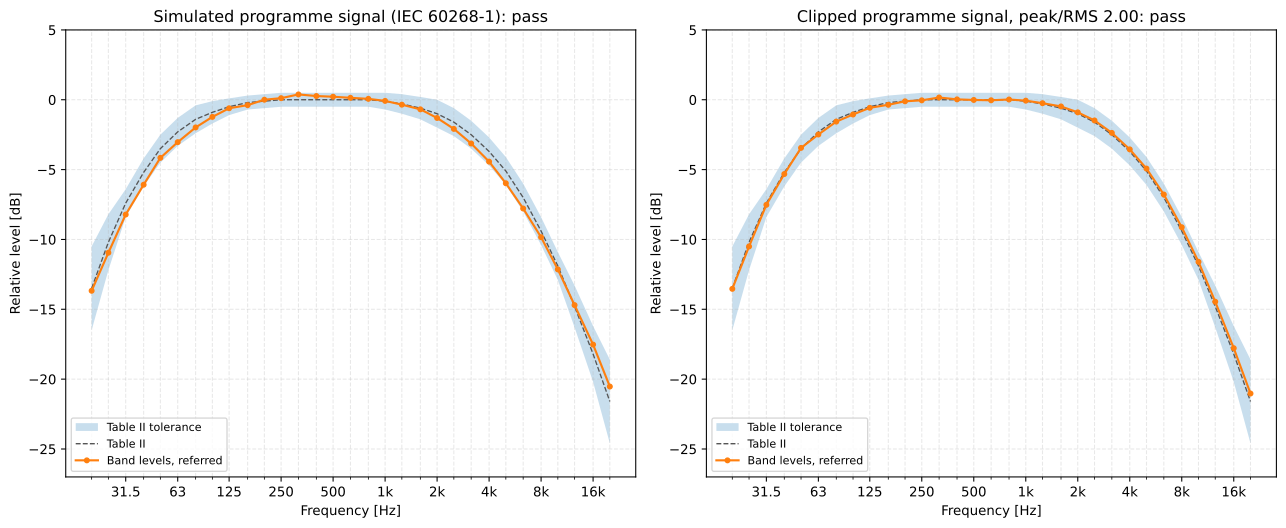
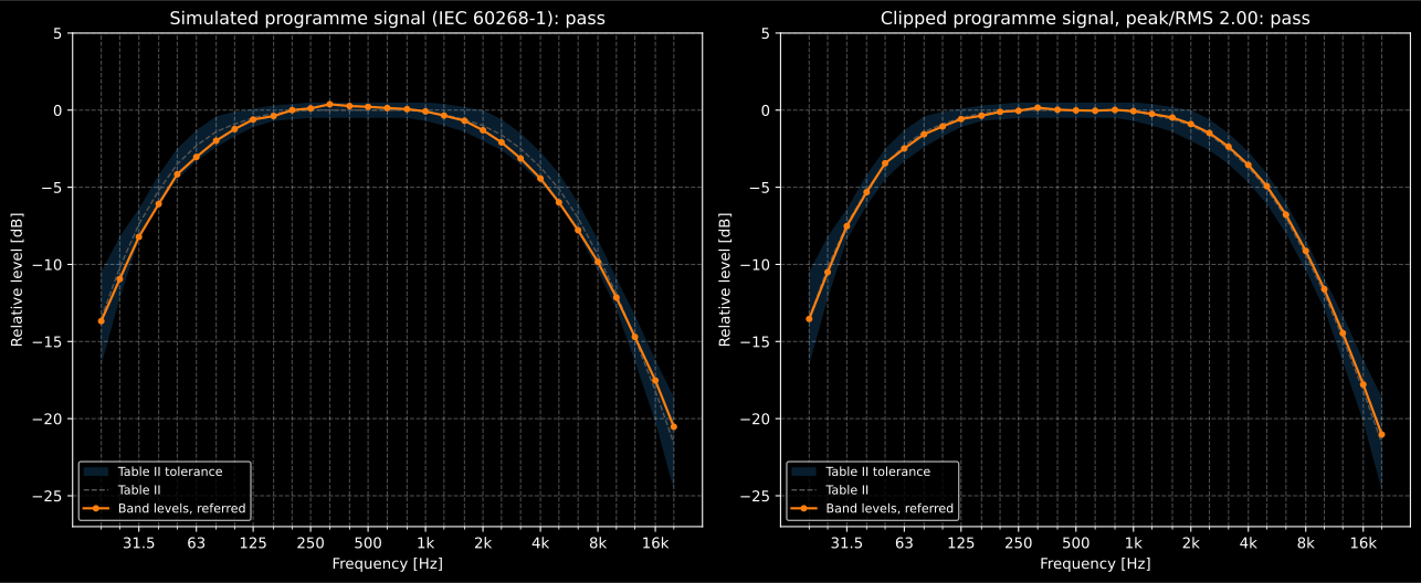
Left, the filter of Figure 2: inside the tolerances, but riding the lower edge on both shoulders of the curve. Right, the generator’s spectrum clipped for the limiting voltages of IEC 60268-7 (section 5), which still follows the table: clipping at twice the RMS value spreads only a little power into the weak upper bands.

import matplotlib.pyplot as plt

clipped = electroacoustics.simulated_programme_signal(fs, 60.0, peak_to_rms=2.0, seed=2)
limiting = electroacoustics.check_limiting_test_signal(clipped, fs)
fig, (ax_figure_2, ax_limiting) = plt.subplots(1, 2, figsize=(13.5, 5.6))
check.plot(ax_figure_2)
limiting.plot(ax_limiting)
plt.show()

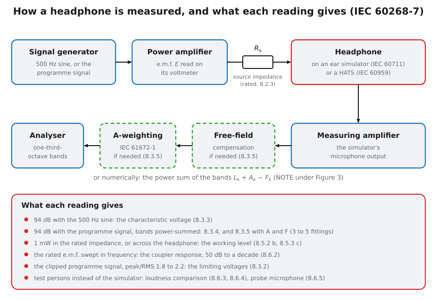
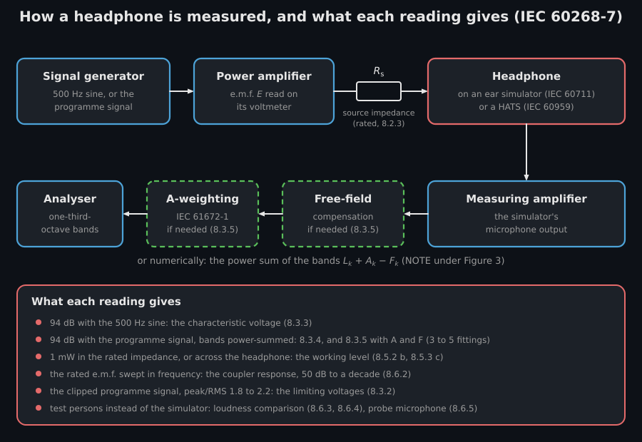
1. The standard conditions (7.2, 7.3). One earphone sits at its rated application force on the coupler or ear simulator its standard names (IEC 60318, IEC 60711, or the ear of the head and torso simulator of IEC 60959, with the pinna simulator of Annex A where it applies), and the type is stated with the results. The signal is a source e.m.f. applied through the rated source impedance, 120 Ω for a headphone output by IEC 61938, at the point an amplifier drives in use, and set for 94 dB at the standard measuring frequency of 500 Hz; the manufacturer may set 1 mW in the rated impedance instead. Volume controls sit at minimum attenuation.
2. With the programme signal (7.4, Figure 3). The same, with the simulated programme signal of IEC 60268-1 from a generator and a power amplifier whose voltmeter reads the e.m.f.; the simulator’s output passes, where a clause asks for it, through the A-weighting of IEC 61672-1 and a filter with the inverse of the head and torso simulator’s free-field response, then a one-third-octave analyser. The NOTE under the figure allows the same correction numerically, which is what section 5 does. A noise reading wanders, so it is repeated and averaged (8.3.4.2 NOTE 2), and for 8.3.5 the headphone is taken off and put back between 3 to 5 readings.
3. With test persons (7.5, 7.6). The comparison responses put a listener in a free field, a progressive plane wave (7.5.2), or in a diffuse field (7.5.3), and ask for equal loudness band by band; the ear canal responses put a probe microphone that meets Annex B at least 4 mm inside the canal and read levels instead. Annexes C to E give the practical details.

IEC 60268-7 names a headphone by a code, 60268-7-IEC-XXXX-NNRN-N: four letters for the principle of the transducer, the type of earphone, the acoustic coupling to the ear canal and the radiation to the outside, the impedance in ohms in “mantissa and exponent” form, and the number of channels. The clause gives three impedances, 8 Ω as 08R0, 32 Ω as 32R0 and 600 Ω as 06R2; the last one settles the choice the rule leaves open, between 06R2 and 60R1, in favour of giving every trailing zero to the exponent.

code = electroacoustics.HeadphoneClassification("D", "C", "S", "C", 32.0, 2).code
print(code)  # 60268-7-IEC-DCSC-32R0-2
print([electroacoustics.impedance_code(ohm) for ohm in (8, 32, 600, 150)])
# ['08R0', '32R0', '06R2', '15R1']
earbud = electroacoustics.parse_classification_code("60268-7 - IEC - DELO - 16R0 - 2")
print(earbud.description)
# electrodynamic (moving coil), intra-concha, acoustically open (controlled
# leakage), open-back

The rated impedance is a pure resistance the manufacturer states, “chosen so that the lowest value of the modulus of the actual impedance within the rated frequency range is not less than 80 % of the rated value”; a dip below that anywhere up to 20 kHz should be stated, and the modulus is measured “at least over the frequency range 20 Hz to 20 kHz”. verify_rated_impedance judges the first, lists the second and checks the third.

f = np.geomspace(10.0, 30000.0, 241)
z = 31.0 + 22.0 / (1.0 + ((f / 90.0 - 90.0 / f) / 0.9) ** 2) + 4.0 * (f / 20000.0)
impedance = electroacoustics.verify_rated_impedance(
    f, z, rated_impedance_ohm=32.0, rated_frequency_range_hz=(15.0, 25000.0)
)
print(impedance.passes, round(impedance.minimum_ohm, 1), round(impedance.minimum_ratio, 3))
# True 31.3 0.979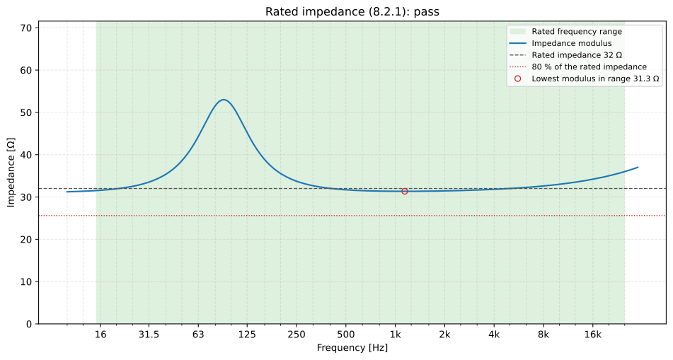

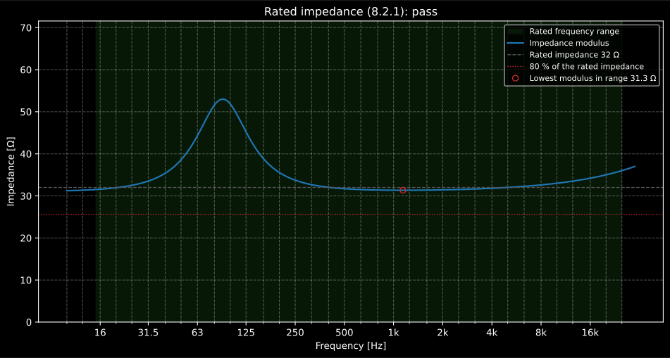
The coil’s resistance sets the floor, the moving system’s resonance the peak and the coil’s inductance the rise. The minimum, 31.3 Ω, is 98 % of the rated 32 Ω, well clear of the 80 % the clause allows.

ax = impedance.plot()
plt.show()

Every input of IEC 60268-7 is a source e.m.f. applied through the rated source impedance, 120 Ω for a headphone output by IEC 61938 (7.1 NOTE). The characteristic voltage (8.3.3) is the 500 Hz sinusoidal e.m.f. that produces 94 dB in the coupler or ear simulator; the headphone is linear there, so one reading scales to it. Every voltage has a power counterpart (8.4), the power it would dissipate in a resistance equal to the rated impedance through the rated source impedance, $P=E^{2}R/(R+R_{\mathrm{s}}{)}^2$, and the working sound pressure level (8.5.2) is the level at the e.m.f. that dissipates 1 mW that way.

characteristic = electroacoustics.characteristic_voltage(0.1, 100.0)
print(round(characteristic, 4))  # 0.0501 V
impedances = {"rated_impedance_ohm": 32.0, "rated_source_impedance_ohm": 120.0}
print(round(electroacoustics.headphone_source_emf(1e-3, **impedances), 3))  # 0.85 V
print(round(1e3 * electroacoustics.headphone_input_power(5.0, **impedances), 1))
# 34.6 mW from the 5 V rated source e.m.f. of 8.3.1 NOTE 2
print(round(20 * np.log10(5.0 / characteristic), 1))  # 40.0 dB above it

8.3.1 NOTE 3 draws attention to hearing damage and says the rated source e.m.f. “should, preferably, not exceed the characteristic voltage (see 8.3.3) by more than 10 dB to 15 dB”. The 5 V of IEC 61938 on this headphone sits 40 dB above it. NOTE 3 states a preference over a range, so the number is yours to read; the library gives no verdict on it.

The simulated programme signal characteristic voltage (8.3.4) is the same 94 dB with the programme signal, and 8.3.5 reads it after the A-weighting of IEC 61672-1 and the inverse of the head and torso simulator’s free-field response. The NOTE under Figure 3 does without filters: the one-third-octave band levels in the ear simulator are multiplied by the filters’ coefficients and power-summed,

with $A_k$ the A-weighting at the exact centre of band $k$ and $F_k$ the free-field response. 8.3.5 g) removes and refits the headphone between readings and averages the e.m.f. of 3 to 5 fittings.

centres = np.array(list(table))
in_range = (centres >= 100.0) & (centres <= 10000.0)
bands_hz = centres[in_range]
resonance = 9.0 / (1.0 + ((bands_hz / 3000.0 - 3000.0 / bands_hz) / 0.8) ** 2)
reading = 72.0 + levels[in_range] + resonance  # dB re 20 µPa at 0.1 V
fittings = np.vstack([reading, reading + 0.6, reading - 0.4])
plain = electroacoustics.programme_characteristic_voltage(0.1, bands_hz, fittings)
weighted = electroacoustics.programme_characteristic_voltage(
    0.1, bands_hz, fittings, a_weighted=True
)
print(round(plain.characteristic_voltage_v, 3), round(weighted.characteristic_voltage_v, 3))
# 0.241 0.253
print(weighted.fittings_conform)  # True, three fittings
working = electroacoustics.working_sound_pressure_level(plain.levels_db[0], 0.1, **impedances)
print(round(working, 1))  # 104.9 dB at 1 mW

The weighted call stops at the A-weighting. 8.3.5 also compensates the free-field response of the head and torso simulator of IEC 60959, which is that manikin’s own data and not a table the library holds; a real 8.3.5 reading passes it as free_field_response_db. The 0.253 V is therefore the e.m.f. for 94 dB A-weighted only, not the corrected characteristic voltage of 8.3.5, and the figure says so in its title.

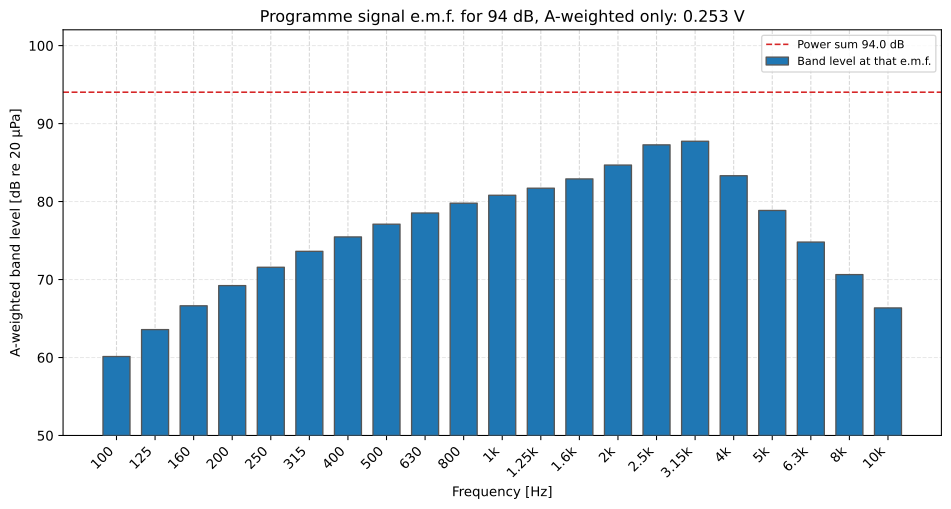
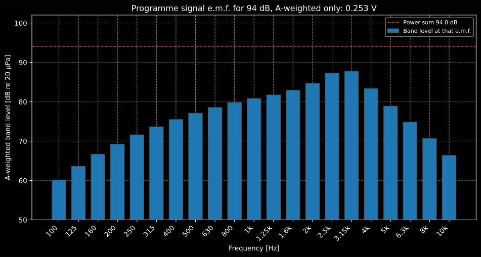
The band levels at the e.m.f. that gives 94 dB A-weighted: their power sum is 94 dB, carried mostly by the four bands around the ear simulator’s canal resonance near 3 kHz. With the free-field compensation of a head and torso simulator as well, the same call gives the corrected characteristic voltage of 8.3.5.

ax = weighted.plot()
plt.show()

The method of 8.5.3 c) sets the 1 mW e.m.f. another way, so that the voltage across the headphone’s own input connector is the one that would put 1 mW into the rated impedance. The two agree only when the headphone presents its rated impedance at 500 Hz. Given the measured impedance, working_sound_pressure_level gives the method’s reading as well; for a 32 Ω headphone that is 40 Ω at 500 Hz it is 1.49 dB lower, and the errata register records the disagreement.

by_definition = electroacoustics.working_sound_pressure_level(100.0, 0.5, **impedances)
by_method = electroacoustics.working_sound_pressure_level(
    100.0, 0.5, **impedances, headphone_impedance_ohm=40.0
)
print(round(by_definition, 2), round(by_method, 2))  # 104.61 103.11

The limiting voltages of 8.3.2 are the e.m.f.s a headphone survives, for ten minutes of one-minute bursts or for 100 h, of the programme signal “with additional clipping”: its spectrum still that of IEC 60268-1, its peak-to-RMS ratio “between 1,8 and 2,2”. That window is IEC 60268-7’s own: IEC 60268-1 asks for noise “without amplitude limiting” and specifies no crest factor, whatever NOTE 1 of 8.3.4.2 says. peak_to_rms clips the generator to exactly that ratio, and check_limiting_test_signal judges a record on both counts.

print(round(limiting.peak_to_rms, 2), limiting.passes)  # 2.0 True
unclipped = electroacoustics.check_limiting_test_signal(y, fs)
print(round(unclipped.peak_to_rms, 2), unclipped.passes)  # 4.92 False

A protective device “causes a change of at least 1 dB in the sensitivity” at its protection voltage, and the impedance and level are then measured 1 dB below and 1 dB above it. protection_voltage takes a sweep of e.m.f. and level, reads the sensitivity at each step against the first, and interpolates where the change reaches 1 dB.

emf = np.array([0.1, 0.2, 0.5, 1.0, 1.5, 2.0, 3.0, 5.0])
shortfall = np.array([0.0, 0.0, 0.05, 0.2, 0.7, 1.6, 3.5, 7.0])
protection = electroacoustics.protection_voltage(
    emf, 94.0 + 20 * np.log10(emf / 0.1) - shortfall
)
print(round(protection.protection_voltage_v, 2))  # 1.65 V
print([round(v, 2) for v in protection.measurement_voltages_v])  # [1.47, 1.85]

The coupler or ear simulator frequency response (8.6.2) is the level against frequency at the rated e.m.f., over at least the rated frequency range, and its graph is drawn with “the same length representing 50 dB as represents one decade of frequency”. The crosstalk attenuation (8.12) is the difference between the level in a channel’s coupler driven by that channel and by another.

fr = np.geomspace(20.0, 20000.0, 241)
level = (
    104.0
    - 10.0 * np.log10(1.0 + (60.0 / fr) ** 4)
    + 6.0 / (1.0 + ((fr / 3200.0 - 3200.0 / fr) / 0.6) ** 2)
    - 10.0 * np.log10(1.0 + (fr / 12000.0) ** 6)
)
response = electroacoustics.coupler_frequency_response(
    fr, level, rated_frequency_range_hz=(20.0, 20000.0)
)
crosstalk = electroacoustics.crosstalk_attenuation(
    bands_hz, np.full(bands_hz.size, 100.0), 52.0 - 12.0 * np.log10(bands_hz / 1000.0) ** 2
)
print(response.covers_rated_range, round(crosstalk.minimum_db, 1))  # True 48.0

None of these responses has a tolerance: “It is not at present possible to set limits for the frequency range based on deviations from a flat, or defined, frequency response” (8.6.6 NOTE 2). The rated frequency range is the manufacturer’s statement, with the criteria its limits were chosen by, and enters here only as the range a measurement has to cover.

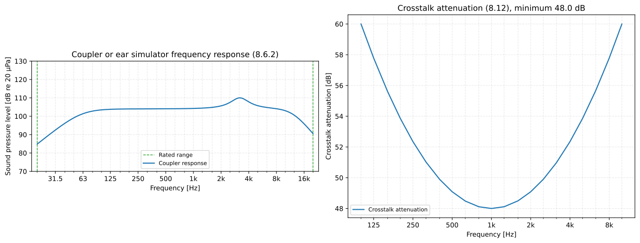
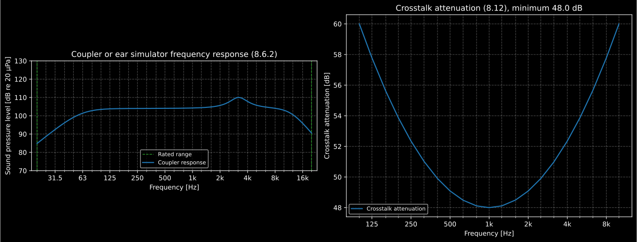
At 50 dB to the decade a coupler response looks as flat as the ear hears it: the 6 dB peak near 3 kHz, which a stretched axis turns into a mountain, is a modest bump.

fig, (ax_response, ax_crosstalk) = plt.subplots(1, 2, figsize=(13.5, 5.2))
response.plot(ax_response)
crosstalk.plot(ax_crosstalk)
plt.show()

The other responses are measured with test persons. In the comparison methods (8.6.3, 8.6.4) each person adjusts the e.m.f. until the headphone is as loud as a free or diffuse reference field in each one-third-octave band of pink noise; the response is the field’s sound pressure over that e.m.f., “expressed in decibels referred to the value at the standard reference frequency”, averaged over at least eight persons with the standard deviation in each band, and a headphone measured on at least 16 may serve as the reference of the substitution method. The ear canal method (8.6.5) puts a probe microphone in the ear canal instead of asking for a judgement, and reads Formula (1),

after averaging two fittings of the headphone and two readings of the sound field, with the procedure repeated when the fittings differ by more than 2.5 dB in any band and the 500 Hz band matched to the field’s within 3 dB; 16 persons calibrate the headphone that replaces the sound field of the indirect method (8.6.5.3).

The two use different reference bands. Formula (1) prints its own, 500 Hz, the standard measuring frequency of 7.2 b). “The standard reference frequency” of the comparison responses is a term IEC 60268-7 never defines; IEC 60268-1 Clause 3, which it cites, sets it at 1 000 Hz “in the absence of a clear reason to the contrary”, the band 8.6.3.2 c) begins and ends the test sequence on, so field_comparison_response refers to 1 kHz unless it is given reference_frequency_hz.

rng = np.random.default_rng(7)
shape_db = 3.0 / (1.0 + ((bands_hz / 2500.0 - 2500.0 / bands_hz) / 0.7) ** 2)
equal_loudness_emf = 0.05 * 10.0 ** (
    -(shape_db + rng.normal(0.0, 1.2, (8, bands_hz.size))) / 20.0
)
comparison = electroacoustics.field_comparison_response(
    bands_hz, 70.0, equal_loudness_emf, field="free"
)
field = 70.0 + rng.normal(0.0, 0.4, (8, 2, bands_hz.size))
earphone = field + shape_db + rng.normal(0.0, 0.6, (8, 2, bands_hz.size))
ear_canal = electroacoustics.ear_canal_frequency_response(bands_hz, earphone, field)
band = list(bands_hz).index(2500.0)
print(comparison.meets_panel_size, round(comparison.mean_db[band], 1))  # True 2.8
print(round(ear_canal.mean_db[band], 1), ear_canal.fittings_consistent.all())  # 3.2 True
print(comparison.reference_frequency_hz, ear_canal.reference_frequency_hz)  # 1000.0 500.0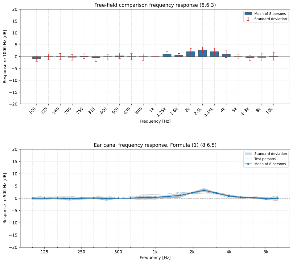

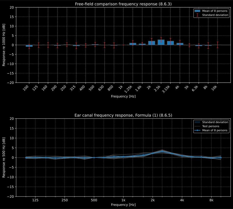
The same headphone through two panels, at the 50 dB to the decade the part prefers, where a 3 dB rise is the modest bump it is. The loudness judgements scatter by 0.7 dB to 1.6 dB in every band but the reference; the probe microphone, which needs no judgement, scatters by 0.2 dB to 0.8 dB and shows the same 3 dB rise at 2.5 kHz.

fig, (ax_comparison, ax_ear) = plt.subplots(2, 1, figsize=(10, 9.6))
comparison.plot(ax_comparison)
ear_canal.plot(ax_ear)
plt.show()

The distortions of a headphone are the ones of IEC 60268-2, read with harmonic_distortion, modulation_distortion and difference_frequency_distortion and expressed as $20\lg$ of the ratio. What IEC 60268-7 adds are the signals. For modulation distortion, 70 Hz and 600 Hz in the amplitude ratio 4:1 with the peak of the rated input voltage, “−1,9 dB at 70 Hz and −14,0 dB at 600 Hz” (NOTE 1 of 8.7.3.3); for difference-frequency distortion, two tones 80 Hz apart, each at half the rated input voltage. Both generators start every tone at its crest, so the sum reaches the rated peak. Below, a drive with a little square law in it puts the second-order product of the two tones at 80 Hz, 35.1 dB under them.

modulation = electroacoustics.headphone_modulation_signal(fs, 1.0, rated_source_emf_v=1.0)
products = electroacoustics.modulation_distortion(modulation, fs, f_low=70.0, f_high=600.0)
print(round(float(np.max(np.abs(modulation))), 4))  # 1.4142, the peak of 1 V RMS
print(products.sideband_frequencies)  # [460. 530. 670. 740.]
difference = electroacoustics.headphone_difference_frequency_signal(
    fs, 1.0, upper_frequency_hz=1000.0, rated_source_emf_v=1.0
)
driven = difference + 0.05 * difference**2  # a drive with 5 % of square law
second = electroacoustics.difference_frequency_distortion(driven, fs, f1=920.0, f2=1000.0)
print(round(20 * np.log10(second), 1))  # -35.1 dB, the product at 80 Hz

The third-order products are at 460 Hz and 740 Hz, as item b) of 8.7.3.3 says. Formula (3) under it prints $U_{470}$, and Formula (5) of the difference-frequency distortion closes a parenthesis it never opened; the errata register records both, with the cross-references of 8.6.3 to 8.6.5 and of Table 1 that name the wrong subclause, the NOTE under Figure 3 that cites the head and torso simulator as IEC 60969, the NOTE of 8.3.4.2 that credits IEC 60268-1 with a crest factor, and the two settings of the 1 mW e.m.f. in 8.5.2 b) and 8.5.3 c).

The microphone in the ear canal of 8.6.5 is specified by the normative Annex B: a cross-sectional area of 5 mm² or less in the concha and the first 4 mm of the canal, less than 0.6 of the canal’s area beyond (an adult’s averages 45 mm²), a volume under 130 mm³, responses to neighbouring one-third-octave bands of pink noise within 3 dB of each other, and an output at least 15 dB lower with the entrance sealed. verify_ear_canal_microphone judges all five.

microphone = electroacoustics.verify_ear_canal_microphone(
    entrance_area_mm2=3.8,
    canal_section_area_mm2=19.0,
    volume_mm3=95.0,
    pink_noise_band_levels_db=[61.0, 62.2, 63.1, 62.5, 61.4],
    open_levels_db=[62.0, 63.0, 62.5],
    sealed_levels_db=[41.0, 44.0, 45.5],
)
print(microphone.passes, round(microphone.area_ratio, 3))  # True 0.422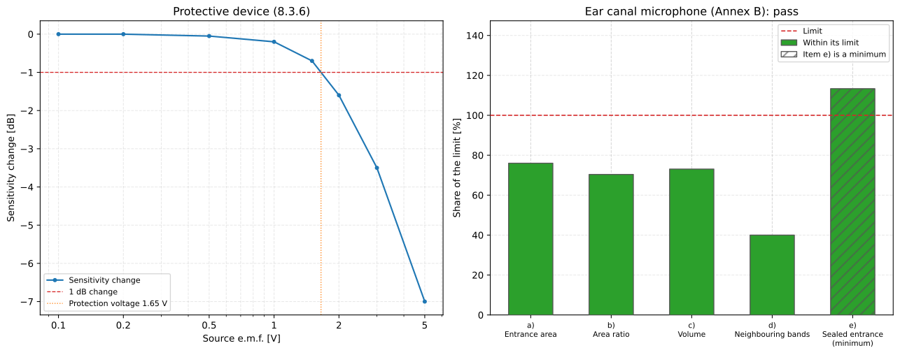

Left, a limiter that cuts in gently: the sensitivity has lost 1 dB at 1.65 V, where 8.3.6.2 b) reads the protection voltage. Right, the probe microphone of Annex B: four upper limits met with room to spare, and the sealed entrance 17 dB down against the 15 dB required.

fig, (ax_protection, ax_microphone) = plt.subplots(1, 2, figsize=(13.5, 5.4))
protection.plot(ax_protection)
microphone.plot(ax_microphone)
plt.show()

• Covered

  IEC 60268-1:1985 Clause 7 with its two amendments of 1988: Table II and its Note, the filter of Figure 2 as an exact transfer function, a generator of the programme signal with the table’s band levels or through the filter, optionally clipped to a peak-to-RMS ratio, and the verdict on a one-third-octave spectrum. IEC 60268-7:2010: the classification code of Clause 4; the rated impedance and the measured range of 8.2; the characteristic voltage (8.3.3), the programme signal characteristic voltages of 8.3.4 and 8.3.5 by the power summation of the NOTE under Figure 3 with the averaging of 3 to 5 fittings, the clipped programme signal of the limiting voltages (8.3.2.2 b) and the protection voltage (8.3.6.2 b); the powers of 8.4 and the working sound pressure levels of 8.5.2, by the definition or by the method of 8.5.3 c); the coupler or ear simulator response (8.6.2), the free-field and diffuse-field comparison responses with their panel sizes, referred to the standard reference frequency of IEC 60268-1 Clause 3 (8.6.3, 8.6.4), the ear canal response by Formula (1) with its fitting and level checks and the 16 persons of a reference (8.6.5); the distortion test signals of 8.7.3 and 8.7.4; the sound attenuation of 8.11, which is ISO 4869-1 and is computed by hearing.real_ear_attenuation, with hearing.anr_total_attenuation of ISO 4869-6 for a headphone with active noise compensation; the crosstalk attenuation (8.12); and the probe microphone of Annex B, items a) to e).

• Not covered

  The rated conditions (7.1, 8.6.6, 8.8, 8.13, 8.14) are stated by the manufacturer, the frequency responses carry no tolerance to judge (8.6.6 NOTE 2), and the endurance runs of 8.3.2 are a test schedule, not a computation. The preference of 8.3.1 NOTE 3, a rated source e.m.f. no more than 10 dB to 15 dB above the characteristic voltage, is a range, so it gets a number and no verdict. The external field (8.9) and the unwanted sound radiation (8.10) are readings. The free-field response of the head and torso simulator of IEC 60959 is an input, not a table the library holds. Annex A is the geometry of a pinna simulator, and Annexes C to E are informative practical conditions; the sound pressure level limit of 85 dB and the 10 dB signal-to-noise ratio of 8.6.5.2 b) need calibrated readings the response function is not given.

References

Section titled “References”- International Electrotechnical Commission. (1985). Sound system equipment – Part 1: General (IEC 60268-1:1985). With Amendment 1 (1988-01) and Amendment 2 (1988-06), neither of which touches Clause 7. The standard reference frequency of Clause 3, and the simulated programme signal: Clause 7 with its Note, Table II (the power spectrum and its tolerances) and Figure 2 (the filter for a pink-noise source).
- International Electrotechnical Commission. (2010). Sound system equipment – Part 7: Headphones and earphones (IEC 60268-7:2010). Edition 3.0. The classification code (Clause 4), the standard conditions and the measurement with the simulated programme signal (7.2, 7.4, Figure 3 and its NOTE), the impedance (8.2), the voltages (8.3: the limiting values with the clipped programme signal, the characteristic voltage, the programme signal characteristic voltages and the protective devices), the powers (8.4), the sound pressure levels (8.5), the frequency responses (8.6: coupler, free-field and diffuse-field comparison, ear canal Formula (1)), the distortion test signals (8.7), the sound attenuation (8.11, by ISO 4869-1), the crosstalk attenuation (8.12) and the probe microphone of Annex B.
- International Electrotechnical Commission. (2013). Electroacoustics – Sound level meters – Part 1: Specifications (IEC 61672-1:2013). The A-weighting whose band coefficients the NOTE under Figure 3 of IEC 60268-7 sums with, Table 3.
- International Electrotechnical Commission. (2013). Sound system equipment – Part 3: Amplifiers (IEC 60268-3:2013). The difference-frequency distortion of 14.12.8.1 b), the reading Formula (5) of IEC 60268-7 needs where its brackets are unbalanced.