Microphone Calibration by Comparison (IEC 61094-5/-8)
Standards: IEC 61094NPL Report CIRA(EXT) 010Key references: Barham et al. 2014
A working standard microphone is not calibrated by reciprocity. It is put beside a reference microphone whose sensitivity is already known, or in its place, both are exposed to the same sound pressure, and the ratio of their output voltages carries the reference’s sensitivity over to it. IEC 61094-5 does this in a pressure field, in a coupler or a jig; IEC 61094-8 does it in a free field, in an anechoic room or behind a time window. Annex D of the first part writes the model once for both,
where is the ratio of the output voltages of the test and reference
microphones, that of the effective sound pressures acting on them, which
the procedure reduces to unity, and the corrections the part asks for.
metrology.comparison_calibration computes the right-hand form, in
sensitivity levels in dB re 1 V/Pa.
This page runs a pressure calibration of a WS2P against an LS2P and a free-field calibration of a WS2F, with their budgets, then the time-selective processing of IEC 61094-8 Annex B, the phase of the sensitivity, the effect of different acoustic impedances (IEC 61094-5 7.4 and 7.5) with the air between two microphones by the circuit the part refers to, the correction for microphones of different diameters by the model it refers to (6.5), and the validation of a jig or a coupler (6.7); the readings are synthetic, built from sensitivities the page knows, so every step can be checked against them.
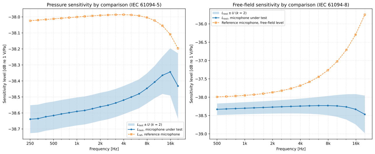
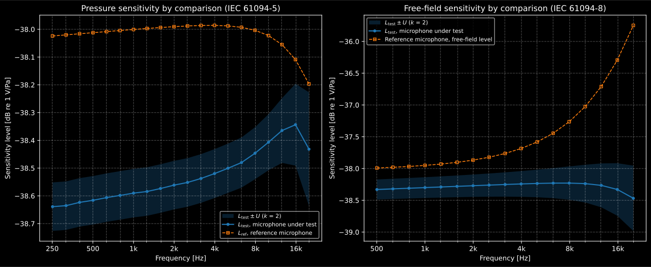
A pressure calibration by simultaneous excitation (left) and a free-field
calibration by substitution (right), from the results’ own .plot().
1. How the measurement goes
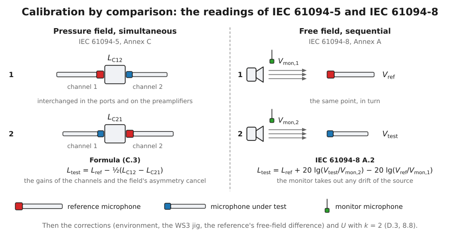
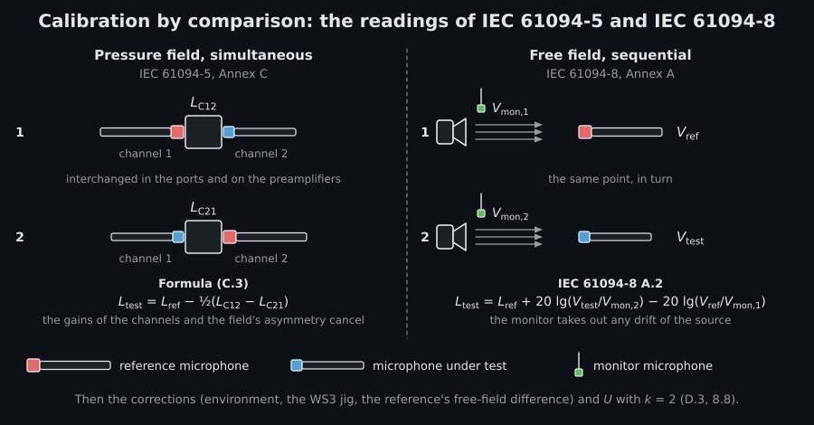
Section titled “1. How the measurement goes”Both parts give two ways of exposing the microphones to the same sound pressure. With simultaneous excitation they sit in the field at once, each read on its own measuring channel; in a coupler or a jig they face each other about 1 mm apart, a small fraction of the wavelength up to 20 kHz (5.1.2). With sequential excitation they take the same place in turn: either the exchange does not change the sound pressure significantly, or any change is detected and corrected, for example with a monitor microphone near the source (5.1.3; IEC 61094-8 5.2, 6.5 and A.2).
| Requirement | Value | Clause |
|---|---|---|
| Reference conditions | 23,0 °C, 101,325 kPa, 50 % relative humidity | 61094-5 and 61094-8, 4 |
| Simultaneous, in a coupler or a jig | Diaphragms about 1 mm apart; the microphones interchanged and the measurement repeated, the result from the two | 61094-5, 5.1.2 |
| Sequential | The exchange does not change the sound pressure significantly, or any change is detected and corrected, for example with a monitor microphone; a monitor, when used, senses the changes at the test position | 61094-5, 5.1.3; 61094-8, 5.2, 6.5 |
| Analysis bandwidth | 1/6 octave or narrower keeps the error below 0,01 dB; much narrower FFT lines can show standing waves | 61094-5, 5.1.1 NOTE |
| Output voltage | Open-circuit, by insert voltage or a high-impedance preamplifier; the method is stated on the certificate | 61094-5, 5.2 |
| Free-field source | 70 dB to 80 dB at the microphone is usually enough; plane progressive waves across the microphone | 61094-8, 6.3 |
| Free-field mounting | On a semi-infinite rod of the microphone’s diameter; LS1P references without their grid | 61094-8, 6.4, 6.7 |
| Reported uncertainty | Expanded, with , at each frequency | 61094-5, 7.9; 61094-8, 8.8 |
2. A pressure calibration by simultaneous excitation
Section titled “2. A pressure calibration by simultaneous excitation”In a coupler the two microphones are read on two channels whose gains are never exactly equal, and the two ports of a coupler never quite see the same pressure. Annex C removes both. With the reference as microphone 1 on channel 1, the level reading difference between the channels is Formula (C.1); after the interchange it is Formula (C.2); and their difference leaves only the two sensitivity levels,
so . Here the channels differ by 0,55 dB, port A hears up to 0,13 dB more than port B, and each reading is repeated three times with a little noise:
import numpy as npfrom phonometry import metrology
f = metrology.exact_frequencies(250, 20000, fraction=3)   # 20 exact one-third octavesx = f / 1000l_ref = -38.0 + 0.04 * np.log10(x) - 0.25 * (x / 20) ** 2   # the LS2P's certificate, dB re 1 V/Pal_true = -38.6 + 0.08 * np.log10(x) + 0.2 * (x / 12) ** 2 - 0.5 * (x / 20) ** 4   # the WS2P: unknown
gain_1, gain_2 = 0.35, -0.20      # the two measuring channels, dBfield_a = 0.03 * np.sqrt(x)       # port A of the coupler hears 0.015 dB to 0.13 dB morerng = np.random.default_rng(61094)noise = rng.normal(0.0, 0.004, (2, 3, f.size))   # three repeats of each readingl_c12 = (l_ref + gain_1) - (l_true + gain_2) + field_a + noise[0]   # reference on channel 1l_c21 = (l_true + gain_1) - (l_ref + gain_2) + field_a + noise[1]   # interchanged
c = metrology.simultaneous_comparison(f, l_ref, l_c12, l_c21)print(c.determinations, c.sensitivity_level_db[[2, 8, 19]].round(2))   # 3 [-38.63 -38.58 -38.44]print(np.abs(c.sensitivity_level_db - l_true).max().round(3))           # 0.003
Neither the gains nor the asymmetry reach the result; what is left, 0,003 dB
at most, is the noise of three repeats. 5.1.2 makes the interchange a
requirement for a coupler or a jig, so a pressure calibration without
interchanged_channel_difference_db is refused. The text asks for “the mean
of the two ratios”, and Annex C takes it in decibels: the mean of the two
level differences, which is the geometric mean of the ratios and the only one
in which the gains cancel exactly. The two ratios read before and after the
interchange are 1,1 dB to 1,4 dB apart here, twice the difference of the
channels and of the ports, and their arithmetic mean would sit 0,018 dB to
0,027 dB high.
The environment. A microphone’s sensitivity depends on the static
pressure, the temperature and, for some microphones, the humidity. When the
reference and the test microphone are different models, the reference’s
sensitivity has to be corrected to the conditions of the test (6.6); in a
free field, IEC 61094-8 asks for that correction whatever the models (7.6).
Neither part prints a formula. metrology.environmental_sensitivity_correction
takes the first-order one, a coefficient times a deviation for each
condition, with the coefficients in the units IEC 61094-2 Annex D gives them:
The coefficients are the microphone’s own, which is why they are required: Annex D of IEC 61094-2 puts the low-frequency static pressure coefficient of LS2P microphones between −0,003 dB/kPa and −0,008 dB/kPa and the temperature coefficient within ±0,005 dB/K, and both vary with frequency and from one microphone to the next. 6.5.3 of the same part observes no influence of humidity on a laboratory standard microphone, so that coefficient defaults to 0.
env = metrology.environmental_sensitivity_correction( f, static_pressure_kpa=99.2, # the laboratory during the test temperature_c=21.5, relative_humidity_percent=45.0, static_pressure_coefficient_db_per_kpa=-0.005, # the LS2P's own coefficients temperature_coefficient_db_per_k=0.002,) # from its certificate's 101.325 kPa, 23.0 °C and 50 %print(env.correction_db[0].round(4)) # 0.0076Passed as reference_environment=, the correction is added to the
reference’s level; passed as test_environment=, the test microphone’s own
correction is subtracted from the result, which refers it to the reference
conditions of clause 4 when reliable coefficients are known.
3. The uncertainty budget of Annex D
Section titled “3. The uncertainty budget of Annex D”Table D.1 is a worked budget for a set-up like this one, a low-sensitivity
WS2P against an LS2P in the coupler of Figure A.1 with three repeats, at
2 kHz. That coupler is for frequencies up to 10 kHz (A.1); above, a WS2 goes
in the jig of A.2 and Figure A.3, which reaches 20 kHz. Seven of the eight
rows state a value and how it is read: the reference’s certificate quotes
±0,05 dB with , the capacitance, non-linearity, impedance, drift and
rounding are semi-ranges of rectangular distributions, and the polarising
voltage of (200,0 ± 0,2) V gives a semi-range of
dB. The repeatability row states no
value, only that it was found from the standard uncertainties of a large
number of similar measurements, and prints 0,025 dB as a standard
uncertainty. metrology.IEC61094_5_TABLE_D1 holds each row with its stated
value, its divisor and the standard uncertainty it prints, and the seven that
state a value reproduce it. metrology.comparison_uncertainty_budget combines them on
metrology.combine_uncertainty, every component with a sensitivity of 1 in
the level model, and multiplies by :
d1 = { "reference": 0.025, "capacitance": 0.006, "non_linearity": 0.017, "impedance": 0.003, "polarizing_voltage": 0.005, "repeatability": 0.025, "drift": 0.017, "rounding": 0.003,} # Table D.1, standard uncertainties at 2 kHzb = metrology.comparison_uncertainty_budget(d1, frequency_hz=2000)print(round(b.combined_uncertainty_db, 4), round(b.expanded_uncertainty_db, 3)) # 0.0437 0.087print(round(b.linear_combined_uncertainty_db, 4)) # 0.0436The root-sum-square of the eight printed values is 0,0437 dB, and the
expanded uncertainty 0,087 dB. D.3 prints 0,040 dB and 0,08 dB,
which are not the combination of its own components: 0,040 dB is what the
sum gives with one of the two 0,017 dB rows left out. The case is in the
errata register. D.3 also notes that a
strict calculation would convert each component to linear form before
combining, with essentially the same result, and prints no value for it;
linear_combined_uncertainty_db does it and gives 0,043 614 dB, 0,000 055 dB
below the combination in decibels. The Spanish adoption, UNE-EN
61094-5:2017, leaves six of the eight values of Table D.1 blank and prints
0,004 dB in D.3, which is also in the register.
At other frequencies the components change. 7.9 estimates about 0,1 dB at low and middle frequencies for microphones of the same diameter, rising to about 0,2 dB at 20 kHz for WS2P, and 7.4 and 7.5 name the difference of the microphones’ acoustic impedances as what grows. Here that component rises with frequency, and each budget’s expanded uncertainty goes to the calibration, which the plot draws as a band:
budgets = [ metrology.comparison_uncertainty_budget( {**d1, "impedance": 0.003 + 0.09 * (fx / 20000) ** 2}, frequency_hz=fx ) for fx in f]u = [bb.expanded_uncertainty_db for bb in budgets]c = metrology.simultaneous_comparison( f, l_ref, l_c12, l_c21, reference_environment=env, expanded_uncertainty_db=u)print(np.round(u, 3)[[0, 16, 19]]) # [0.087 0.101 0.205]print(c.sensitivity_mv_per_pa[[2, 8, 19]].round(2)) # [11.72 11.78 11.98]c.plot()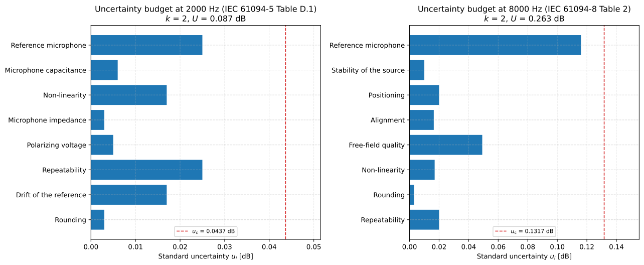
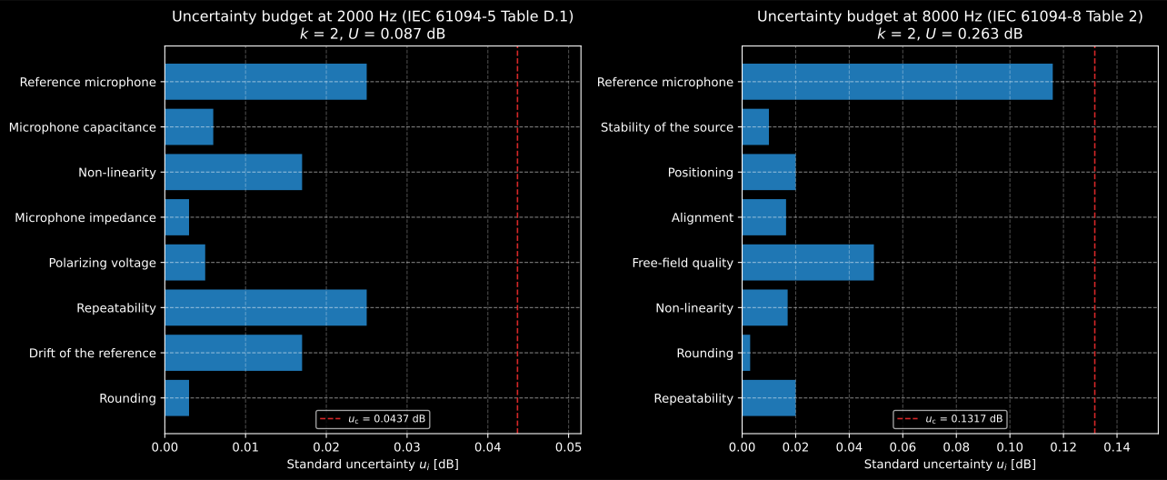
The budget of Table D.1 at 2 kHz (left) and a free-field budget at 8 kHz (right).
4. A WS3 microphone in the jig
Section titled “4. A WS3 microphone in the jig”A WS3 microphone is smaller than the LS2 reference, and in the jig of Figure
A.4 the two diaphragms face each other 0,5 mm apart: the pressure over the
smaller diaphragm is not the mean over the larger one. Table A.1 gives the
corrections to add to the WS3’s sensitivity level, calculated for an LS2aP
reference and a radially symmetrical field and valid for that separation
only, with an expanded uncertainty of a tenth of each correction.
metrology.jig_diameter_correction reads them, and an exact base-ten
frequency reads as its row:
j = metrology.jig_diameter_correction()print(j.correction_db[[0, 9, 13]]) # [-0.004 -0.235 -1.443]print(j.standard_uncertainty_db[13].round(4)) # 0.0722j.correction_db goes to a calibration through corrections_db=, under a
name of its own, and j.standard_uncertainty_db to its budget as an
additional component, the first special case of Table D.1.
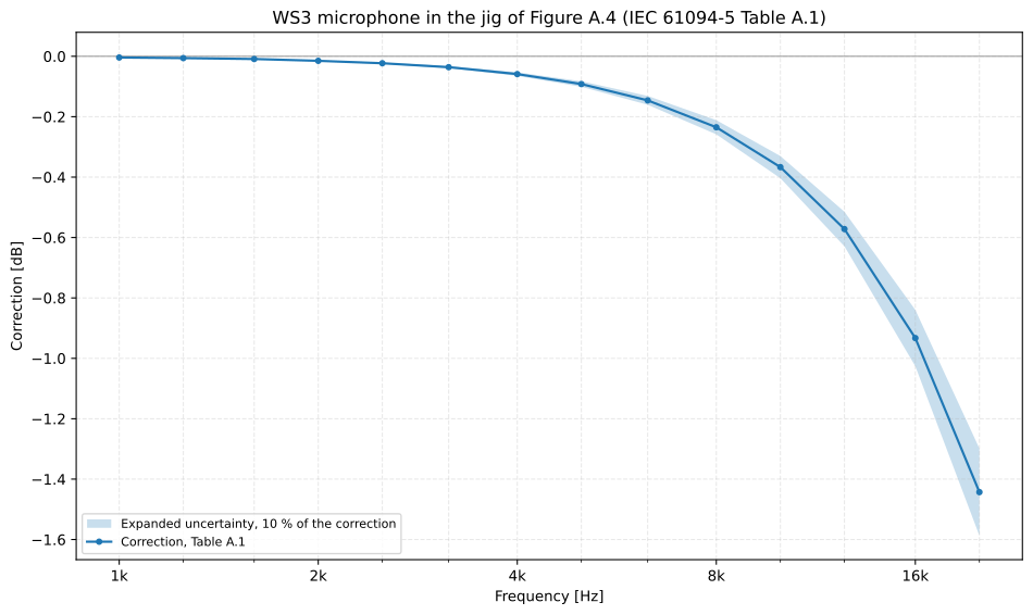
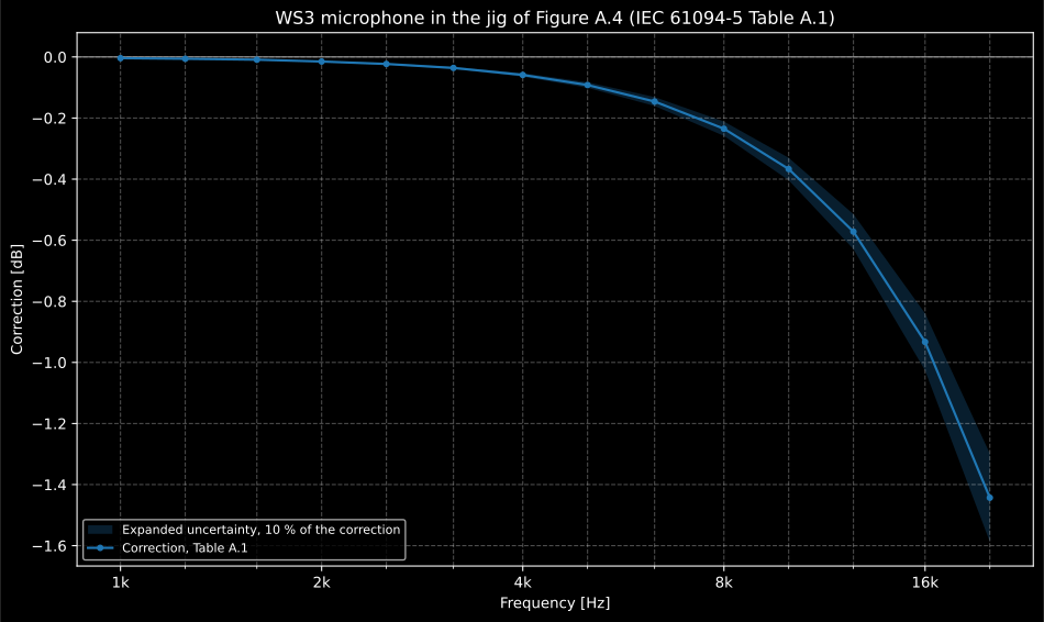
Table A.1 with its expanded uncertainty of 10 %.
Beyond Table A.1: microphones of different diameters
Section titled “Beyond Table A.1: microphones of different diameters”“The effect of a non-uniform pressure distribution over the surface of the diaphragm will be significantly greater if the test and reference microphones are of different diameters. A theoretical model which can be used to apply corrections and assess the uncertainties in this case is given in the literature (for example [1])” (6.5). Its reference [1], Barham, Barrera-Figueroa and Avison (2014), is where Table A.1 comes from. The gap between the diaphragms is a cylinder of the reference’s front-cavity radius and length , closed by the reference at and driven, in a radially symmetrical field, through the annulus round the smaller microphone at . Its pressure is a series of the radial modes of the cavity,
and each microphone reads it averaged over its diaphragm with its radial
sensitivity, the deflection of a membrane under a uniform pressure,
with the
frequency over the diaphragm’s resonance frequency: the reference over
at its face, the test microphone, with in place of , over its
diaphragm across the gap. The correction is the ratio of the two averages,
. metrology.diameter_sound_field_correction
computes it from the geometry and the two resonance frequencies, at the
speed of sound of the IEC 61094-2 Annex F air:
ws3 = { "reference_radius_m": 4.650e-3, # an LS2: its front cavity and diaphragm "test_diaphragm_radius_m": 2.065e-3, # a WS3: its diaphragm "test_outer_radius_m": 2.975e-3, # and its outline "separation_m": 0.5e-3, # Figure A.4 "reference_resonance_frequency_hz": 22000, "test_resonance_frequency_hz": 100000,} # the inputs of Table 1 of [1]model = metrology.diameter_sound_field_correction(j.frequencies_hz, **ws3)print(round(model.speed_of_sound, 1), model.correction_db[[0, 9, 13]].round(3)) # 345.9 [-0.004 -0.233 -1.434]print(np.abs(model.correction_db - j.correction_db).max().round(4)) # 0.0093At the reference air of clause 4 the model is within 0,0093 dB of every row
of Table A.1, inside the 0,144 dB the NOTE gives the largest correction as
its expanded uncertainty. The paper prints no speed of sound; at 344,8 m/s
the model gives every row to the thousandth printed. As printed, the paper’s
formulas with its own inputs do not give its own table: the library reads
the radial sensitivity of its Formula (4) less 1 and the annulus of its
Formula (2) from the WS3’s overall radius, the two readings that do (an
erratum). A.2 sets the expanded uncertainty
of Table A.1 at 10 % of each correction, “which is approximately the change
observed by doubling the distance between the microphones”;
separation_change_db is that change by the model, of the order A.2 states
and below it:
print((model.separation_change_db / np.abs(model.correction_db))[[0, 13]].round(3)) # [0.063 0.054]Table A.1 holds for one pair of microphones at the one separation of Figure A.4, “the only one for which the corrections specified in Table A.1 are valid”, and at fourteen frequencies. The model holds for any test microphone that fits inside its reference’s front cavity, any separation, and any frequency below the two resonance frequencies, where the radial sensitivity it divides by is defined:
f12 = metrology.exact_frequencies(1000, 20000, fraction=12) # every twelfth of an octavefine = metrology.diameter_sound_field_correction(f12, **ws3)print(f12.size, round(f12[50]), fine.correction_db[50].round(3)) # 53 17783 -1.141fine.correction_db goes to a calibration through corrections_db= as
Table A.1 does. The model assumes a radially symmetrical field, which is why
6.5 and A.2 ask for a coaxial source in the far field or a diffuse field.
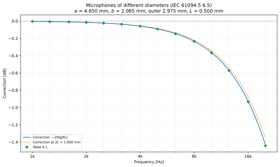
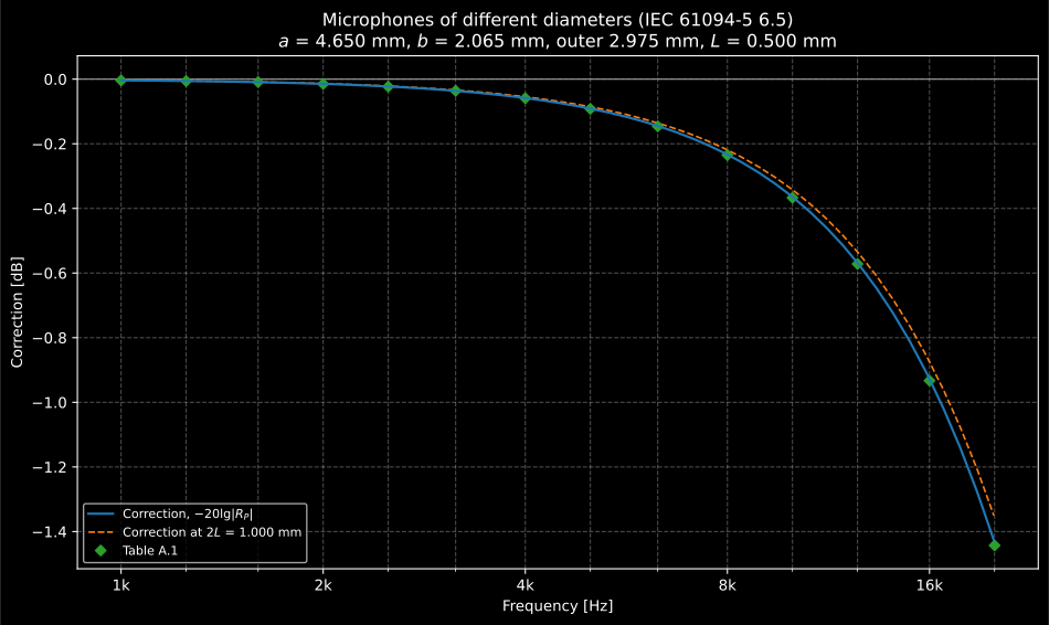
The model of reference [1] for the WS3 in the jig of Figure A.4, with the rows of Table A.1 and the correction at twice the separation.
5. A free-field calibration by substitution
Section titled “5. A free-field calibration by substitution”IEC 61094-8 A.2 describes the basic method: the reference is put at a point
of the free field, then the microphone under test in its place, each read
against a monitor microphone near the source, and “the quotient of these two
gives the ratio of the microphone under test output voltage to the reference
microphone output voltage, corrected for any variation in the sound pressure
generated by the source”. With and the
output voltages of the reference and the monitor in the first reading, and
and those of the second, the monitor’s
two readings going together as a metrology.MonitorReadings,
The reference here is an LS2P calibrated in a pressure field, so its free-field sensitivity is its pressure sensitivity plus the free-field to pressure difference of IEC/TS 61094-7 (Table 1, 8.2). The values below stand in for that difference; take yours from the specification or the microphone’s calibration. Between the two readings the source drifts by 0,25 dB:
ff = metrology.exact_frequencies(500, 20000, fraction=3)xf = ff / 1000c_ff = 0.05 * xf**1.3            # the LS2P's free-field to pressure difference: illustrativel_ref_p = -38.0 + 0.04 * np.log10(xf) - 0.25 * (xf / 20) ** 2   # its pressure calibrationl_ws2f = -38.3 + 0.1 * np.log10(xf) - 0.3 * (xf / 20) ** 3      # the WS2F: unknownfield_1 = 74.0 + 0.05 * np.sin(xf)   # the free field while the reference is in placefield_2 = field_1 + 0.25             # the source has drifted by the time the WS2F ismonitor = -40.0                      # the monitor microphone near the source, dB re 1 V/Pa

def free_field_budget(fx):    x20 = fx / 20000    return metrology.comparison_uncertainty_budget(        {            "reference": 0.06 + 0.14 * x20,    # pressure calibration and IEC/TS 61094-7            "source_stability": 0.01,            "positioning": 0.02,            "alignment": 0.01 + 0.04 * x20**2,            "free_field": 0.03 + 0.12 * x20**2,            "non_linearity": 0.017,            "rounding": 0.003,            "repeatability": 0.02,        },        frequency_hz=fx,        field="free_field",    )

free = metrology.sequential_comparison(    ff,    l_ref_p,    l_ref_p + c_ff + field_1,     # the reference's output, dB re 1 V    l_ws2f + field_2,             # the WS2F's output in its place    monitor=metrology.MonitorReadings(        reference_level_db=monitor + field_1, test_level_db=monitor + field_2    ),    field="free_field",    reference_free_field_difference_db=c_ff,    expanded_uncertainty_db=[free_field_budget(fx).expanded_uncertainty_db for fx in ff],)print(bool(np.abs(free.sensitivity_level_db - l_ws2f).max() < 1e-9))   # Trueprint(free.expanded_uncertainty_db[[0, 12, 16]].round(2))              # [0.16 0.26 0.51]
The monitor takes the drift out exactly; without it the result would be
0,25 dB high at every frequency. Table 2 of IEC 61094-8 lists the typical
components with the subclause that discusses each, and prints no values:
the ones above are illustrative, chosen so that the expanded uncertainty is
near the 0,2 dB 8.8 estimates at low and middle frequencies and the 0,5 dB
it estimates at the upper frequency limit of an LS2 reference.
metrology.IEC61094_8_TABLE_2 holds the list, and
metrology.IEC61094_8_TABLE_1 the typical expanded uncertainty of each way
the reference can be calibrated:
row = metrology.IEC61094_8_TABLE_1["primary_pressure"]print(row.expanded_uncertainty_1khz_db, row.expanded_uncertainty_10khz_db) # 0.12 0.46. The effective free-field region of a time window
Section titled “6. The effective free-field region of a time window”Where the room is not anechoic enough, a time window can keep the direct sound and drop the reflections (6.2.3, Annex B). The window defines the region it simulates a free field in: a prolate spheroid with the source and the microphone at its foci, apart, and the major diameter
where runs from the arrival of the sound at the microphone to the end of the window and is the speed of sound at the prevailing conditions, here from the humid air of IEC 61094-2 Annex F. A reflection from any point of its surface arrives after the direct sound, so every reflecting surface has to be outside it, and so does the far end of the mounting rod:
r = metrology.free_field_region(1.0, 0.005) # 1 m, a 5 ms window, at 23.0 °Cprint(round(r.speed_of_sound, 1), round(r.major_axis_m, 2)) # 345.9 2.73print(round(r.semi_minor_axis_m, 2), round(r.rod_clearance_m, 2)) # 1.27 0.86A 5 ms window at 1 m needs 1,27 m of clearance round the axis mid-way between source and microphone, and a rod that runs more than 0,86 m behind the microphone.
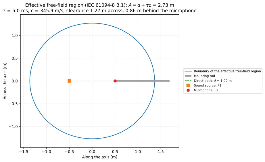
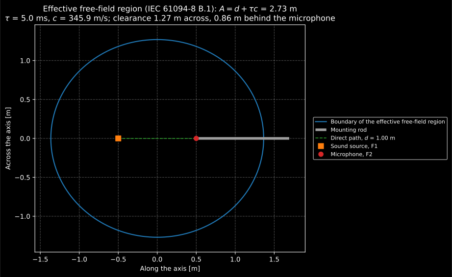
The region of a 5 ms window at 1 m, with the rod that has to leave it.
7. Time-selective processing
Section titled “7. Time-selective processing”Where the room is not anechoic enough, Annex B keeps the direct sound and drops the reflections: an impulse response separates the two in time, a window keeps the first, and a Fourier transform gives the frequency response of the direct sound alone (B.1.1). The impulse response can come from a stepped sine taken to the time domain by the inverse transform,
(metrology.stepped_sine_impulse_response), from a sweep or a maximum length
sequence (room.impulse_response, room.mls_impulse_response), or from a
direct impulse. metrology.time_selective_response weights it with a time
window and evaluates (B.2) at any frequency. “In order not to produce
artefacts in the transformed data, the time window normally has ‘tapered’
edges” (B.1.2); B.1.3 lists Hann, Hamming, Tukey, Butterworth cosine and
Gaussian windows and does not recommend a rectangular one, “because it
usually leads to spectral leakage”. The default is a Tukey window, flat in
the middle with an eighth of it tapered at each edge, a proportion the
library chose, as no clause prints one.
Here an LS2P reference and a WS2F stand in turn 1 m from the source, and a reflection off the rig arrives along a path of 1,48 m. The WS2F hears it off axis, so it does not cancel in the ratio of the two outputs as the direct sound does: “it cannot be assumed that the reference microphone and microphone under test will deviate in the same way” (8.5). Each is measured by a stepped sine from 0 Hz to 100 kHz in 50 Hz steps, past three times the resonance as B.2.1 asks; the microphones are illustrative:
c0 = metrology.free_field_region(1.0, 0.005).speed_of_sound   # 345.9 m/s at 23.0 °Cf_step = np.arange(0.0, 100000.0 + 1.0, 50.0)   # 0 Hz to 100 kHz in 50 Hz steps

def mic(fx, level_db, f0, d):   # a microphone's sensitivity, V/Pa: illustrative    return 10 ** (level_db / 20) / (1 - (fx / f0) ** 2 + 1j * d * fx / f0)

direct, rig = 1.0 / c0, 1.48 / c0   # the direct sound over 1 m, the rig's reflection over 1.48 m

def heard(m, off_axis):   # each step: the direct sound and the rig's reflection    return m * (        np.exp(-2j * np.pi * f_step * direct)        + 0.25 * off_axis * np.exp(-2j * np.pi * f_step * rig)    )

ir_ref = metrology.stepped_sine_impulse_response(f_step, heard(mic(f_step, -38.0, 22000, 1.1), 1.0))ir_ws2f = metrology.stepped_sine_impulse_response(    f_step, heard(mic(f_step, -26.4, 18000, 0.9), 1 / (1 + 1j * f_step / 6000)))   # the WS2F hears the reflection off axisprint(ir_ref.duration_s, round(ir_ref.sample_rate_hz))   # 0.02 200050
The impulse response lasts the inverse of the frequency step, 20 ms. B.2.2
sizes the step by the room: 120 Hz is enough in a small anechoic room
“because the primary reflections all occur before 8 ms”, about 30 Hz in a
large one. (B.2.1 says the increment “will determine the time domain
resolution”; it is the length it sets, as B.2.2 says, and the
errata register records the sentence.)
ir_ws2f.plot() draws the whole record:
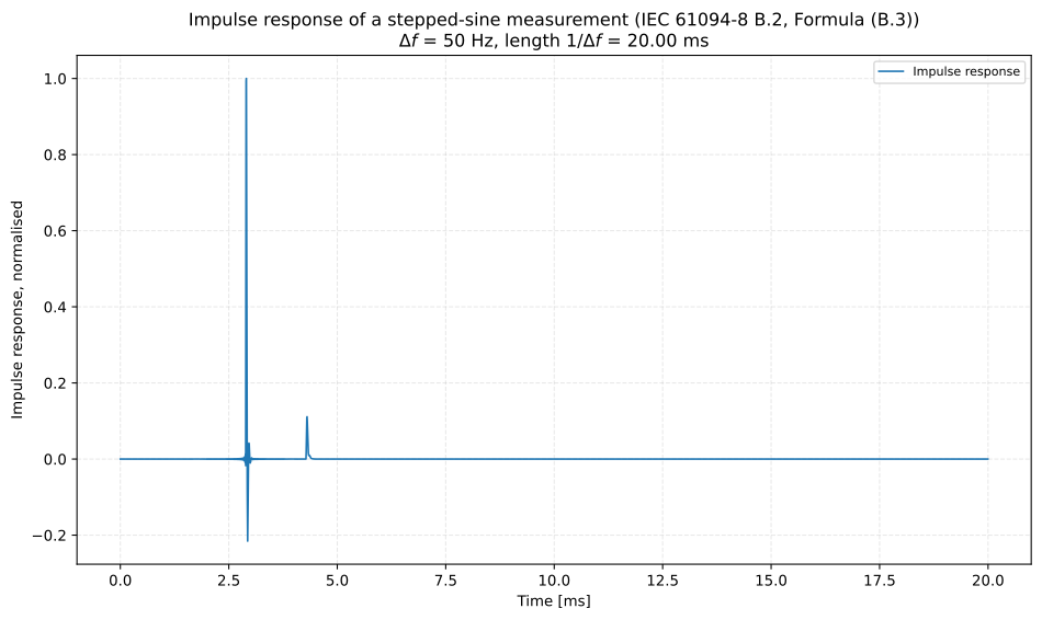
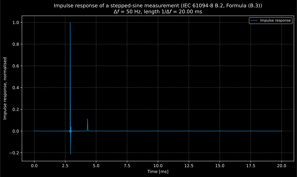
The WS2F’s impulse response from the stepped sine, the whole of
it, from ir_ws2f.plot().
The window has to end before the reflection arrives. A point on the boundary of the region of Formula (B.1) reflects along a path of the major diameter , so a reflection whose path is stays outside while
which metrology.reflection_free_window_s gives, at the speed of sound of
the IEC 61094-2 Annex F air:
tau = metrology.reflection_free_window_s(1.0, 1.48)window = {"window_start_s": direct - 0.0005, "window_end_s": direct + tau}ref = metrology.time_selective_response(ir_ref.impulse_response, ir_ref.sample_rate_hz, **window)ws2f = metrology.time_selective_response(ir_ws2f.impulse_response, ir_ws2f.sample_rate_hz, **window)print(round(1000 * tau, 2), round(ref.frequency_resolution_hz)) # 1.39 530A window of 1,89 ms tells frequencies apart no closer than 530 Hz, the low-frequency limit 6.2.3 warns time-selective techniques have; lower frequencies need another method. The levels and phases through the window are the two outputs of a substitution:
fw = metrology.exact_frequencies(1900, 20000, fraction=3) # 2 kHz to 20 kHzm_ref = mic(fw, -38.0, 22000, 1.1) # the reference's free-field sensitivity, from its certificatetsel = metrology.sequential_comparison( fw, 20 * np.log10(np.abs(m_ref)), ref.level_db_at(fw), ws2f.level_db_at(fw), field="free_field", phase=metrology.SequentialComparisonPhase( reference_sensitivity_phase_deg=np.degrees(np.angle(m_ref)), reference_output_phase_deg=ref.phase_deg_at(fw), test_output_phase_deg=ws2f.phase_deg_at(fw), ),)m_ws2f = mic(fw, -26.4, 18000, 0.9) # what the page knows the WS2F to beprint(tsel.sensitivity_level_db[[0, 6, 10]].round(2)) # [-26.34 -25.46 -26.6 ]print(bool(np.abs(tsel.sensitivity_level_db - 20 * np.log10(np.abs(m_ws2f))).max() < 1e-4)) # Truerecord = 20 * np.log10(np.abs(ws2f.record_response_at(fw) / ref.record_response_at(fw)))print(np.abs(record - 20 * np.log10(np.abs(m_ws2f / m_ref))).max().round(2)) # 1.91Through the window the WS2F’s sensitivity comes back to within 0,0001 dB; from the whole record, the reflection included, it would be up to 1,91 dB off.
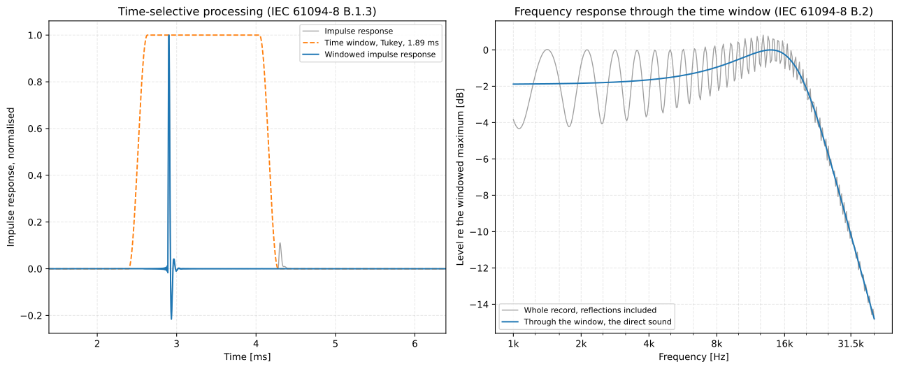
The WS2F’s impulse response with the window over it (left), and its response through the window and from the whole record (right).
The direct impulse method (B.6), which B.6.2 calls “largely superseded”, drives the source with a short rectangular pulse of amplitude . Its spectrum is
whose first zero, , “must be approximately an order of magnitude
higher than the upper limit of the frequency range of interest”. The formula
and its first zero are those of a pulse lasting , although the text calls
the duration (it is in the errata register);
metrology.rectangular_pulse takes the whole duration :
T = metrology.rectangular_pulse_duration_s(20000) # a first zero ten times 20 kHzpulse = metrology.rectangular_pulse(T, amplitude_v=10.0)print(T, pulse.half_duration_s, round(pulse.first_zero_hz)) # 5e-06 2.5e-06 200000print(pulse.level_db_at([20000.0]).round(2)) # [-0.14]The responses to several pulses, averaged synchronously
(signals.time_synchronous_average; B.6.2 counts on dB of
signal-to-noise ratio from of them), go to time_selective_response with
excitation=pulse, which divides the pulse’s spectrum out, as a pulse that
begins at the start of the record.
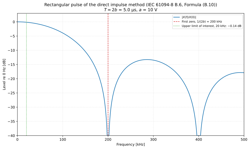
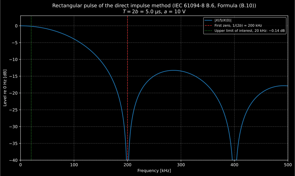
Formula (B.10) for a 5 µs pulse: 0,14 dB down at 20 kHz, the first zero at 200 kHz.
8. The phase of the sensitivity
Section titled “8. The phase of the sensitivity”Both parts carry the phase over with the modulus: IEC 61094-5 5.1.1 calculates “the sensitivity (both modulus and phase) of the test microphone”, and IEC 61094-8 5.1 “both the modulus and phase of the free-field sensitivity of the microphone under test”. D.2 holds for the complex ratios, so the phase follows the level term by term, and the interchange of Annex C cancels the phase shifts of the two channels and of the coupler as (C.3) cancels their gains:
with the phase of channel 1’s reading re channel 2’s. Neither part prints this form; it is (C.3) written for the complex ratio. The pressure calibration of section 2, with the phase of each reading:
phi_ref = np.degrees(np.angle(1 / (1 - (f / 22000) ** 2 + 1.1j * f / 22000))) # the LS2P's certificate: illustrativephi_true = np.degrees(np.angle(1 / (1 - (f / 18000) ** 2 + 0.9j * f / 18000))) # the WS2P: unknownshift_1, shift_2 = 1.5 * x, -0.8 * x # the two channels' phase shifts, degreeslate_a = 0.4 * x # port A hears the field later, degreesjitter = np.random.default_rng(5).normal(0.0, 0.02, (2, 3, f.size))p12 = (phi_ref + shift_1) - (phi_true + shift_2) + late_a + jitter[0] # reference on channel 1p21 = (phi_true + shift_1) - (phi_ref + shift_2) + late_a + jitter[1] # interchangedcp = metrology.simultaneous_comparison( f, l_ref, l_c12, l_c21, phase=metrology.SimultaneousComparisonPhase( reference_sensitivity_phase_deg=phi_ref, channel_phase_difference_deg=p12, interchanged_channel_phase_difference_deg=p21, ),)print(cp.sensitivity_phase_deg[[2, 8, 16, 19]].round(1)) # [ -1.1 -4.6 -35.9 -102.9]print(np.abs(cp.sensitivity_phase_deg - phi_true).max().round(3)) # 0.016The difference of the two readings is twice the phase difference of the
microphones, so it is taken into one turn before it is halved: the result is
unique while they differ by less than 90°. The phase inputs go together, as a
metrology.SimultaneousComparisonPhase here. In a sequential calibration
they are a metrology.SequentialComparisonPhase, the phases of the two
outputs are read against the monitor’s, which go with its levels in its
metrology.MonitorReadings, or against the signal driving the source, and
their quotient is . In a free field
“determination of the phase of the free-field sensitivity requires the
definition of consistent reference phases at the acoustic centres of the
microphones” (IEC 61094-8 5.1). 7.3 positions the centres “at the
measurement points”; in a sequential substitution each goes in turn to the
same point, where is 0, and a delay common to the two readings,
like the travel time from the source in section 7, cancels in their quotient.
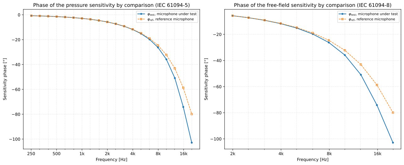
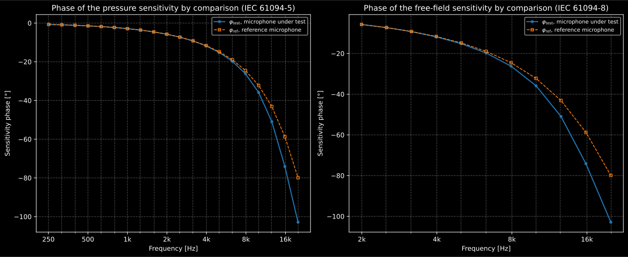
The phase of the WS2P through the interchange (left) and of the WS2F through
the window of section 7 (right), from .plot(quantity="phase").
9. Microphones of different acoustic impedance
Section titled “9. Microphones of different acoustic impedance”“Differences in the acoustic impedance between the test and reference
microphones can cause the sound pressure at the test and reference
microphones to differ” (7.4), most where a pressure and a free-field
microphone meet above 10 kHz, “because of differing volume velocities at the
diaphragms” (7.5). Neither clause prints a model: 7.4 sends the reader to the
literature, and 7.5 asks for the error to be estimated and added to the
budget when no reference of similar impedance is available.
metrology.impedance_pressure_ratio writes the effect for two circuits with
each microphone’s equivalent volume, which IEC 61094-1 6.2.2
defines as with :
In a closed coupler small against the wavelength the source drives the sum
of the admittances of the gas and of every microphone in it, IEC 61094-2
Formula (3), so putting the test microphone in the place of the reference
changes the pressure by the ratio of the two sums, being the rest of
the load: the gas, the source, a monitor. For a simultaneous excitation,
Table D.1 puts “the acoustical impedance of the microphone […] in series
with that of the air in the space between the two microphones”, so that the
two “see slightly different pressures […] (see 7.4 and [2])”: each diaphragm
takes the pressure of a common source behind the same series impedance, and
is the equivalent volume of that impedance, which the circuit of [2]
gives (below). metrology.ReciprocityMicrophone,
the microphone of
the reciprocity calibration,
holds the lumped parameters of IEC 61094-2 E.4, the low-frequency volume, the
resonance frequency and the loss factor, and its
complex_equivalent_volume_m3 gives from them. Its ratio to
the low-frequency volume holds no , so with the 10 mm³
that Table 3 of IEC 61094-1 gives an LS2P, is the volume of
6.2.2 with its 1,40. E.4 finds the representation “of sufficient accuracy” up
to “about 1,3 times the resonance frequency of the microphone”: 20,8 kHz for
the WS2F below, so the example stays within it. The front cavity the
microphone also holds enters the transfer impedance of a coupler, not
.
fi = metrology.exact_frequencies(1000, 20000, fraction=3)front = {"front_cavity_volume_m3": 34e-9, "front_cavity_depth_m": 0.5e-3, "front_cavity_diameter_m": 9.3e-3} # an LS2aP's (Table C.1 of IEC 61094-2)lumped_ls2p = metrology.ReciprocityMicrophone( equivalent_volume_m3=10e-9, resonance_frequency_hz=22000, loss_factor=1.1, **front) # an LS2P: 10 mm³ (IEC 61094-1 Table 3); the resonance and loss: illustrativelumped_ws2f = metrology.ReciprocityMicrophone( equivalent_volume_m3=30e-9, resonance_frequency_hz=16000, loss_factor=0.5, **front) # a more compliant WS2F: illustrativerp = metrology.impedance_pressure_ratio( fi, reference_equivalent_volume_m3=lumped_ls2p.complex_equivalent_volume_m3(fi), test_equivalent_volume_m3=lumped_ws2f.complex_equivalent_volume_m3(fi), coupling_equivalent_volume_m3=600e-9, # the coupler's gas, source and monitor: illustrative)print(rp.level_difference_db[[0, 10, 13]].round(3)) # [-0.281 -0.421 0.37 ]print(rp.standard_uncertainty_db[[0, 10, 13]].round(3)) # [0.163 0.243 0.213]A monitor that “shall accurately sense changes in the sound pressure at the
test/reference microphone position” (5.1.3) takes this ratio out. Without
one, rp.level_difference_db and rp.phase_difference_deg go to the
comparison as pressure_level_difference_db and as the
pressure_phase_difference_deg of its phase inputs. Where the ratio is estimated rather than
corrected for, rp.standard_uncertainty_db is the "impedance" component of
the budget: the level difference read as the semi-range of a rectangular
distribution, as Table D.1 reads its 0,005 dB at 2 kHz, “equivalent to a
standard uncertainty of 0,005/√3 dB = 0,003 dB”. The same row warns about
exactly this pairing: “When microphones have significantly differing
impedances (for example WS2F microphone compared against LS2P at frequencies
above 10 kHz), the measurement uncertainty can be considerably larger and
should be established experimentally.” Above 10 kHz the value here is the
model’s estimate, not that experiment; where the ratio crosses 0 dB, near
16 kHz, it gives almost nothing at all.
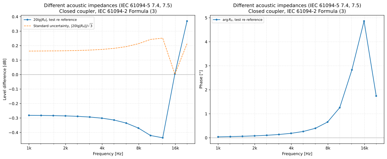
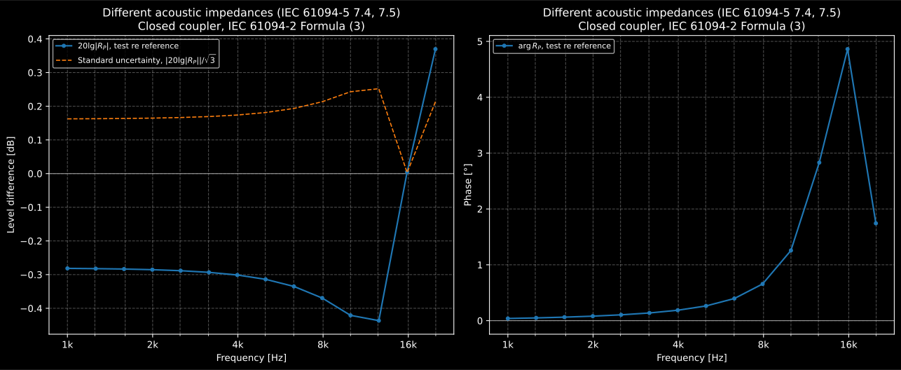
A WS2F in the place of an LS2P in a closed coupler: the level of with its semi-range read as a standard uncertainty (left), which above 10 kHz Table D.1 asks to be established experimentally, and its phase (right).
The air between the two microphones
Section titled “The air between the two microphones”The “Microphone impedance” row of Table D.1 refers the simultaneous excitation to its reference [2], Jarvis (1996), NPL Report CIRA(EXT) 010. Its Appendix B models a symmetric coupler as a ladder from a source in its middle: on each side a mass , the compliance of that side’s half of the volume, a second and the microphone, for a tube of length and radius ,
Seen from each diaphragm, the middle of the ladder is a pressure common to both behind one impedance,
so each diaphragm takes , the divider
above, and the ratio of the two is the one Appendix B prints.
metrology.air_gap_series_impedance_pa_s_m3 gives for a coupler of
known length and radius, at the air of the conditions given. Appendix B’s
example is an LS2P against a high sensitivity WS2P in a tube 2 mm long and
12,7 mm across, each microphone a resistance, a mass and a compliance in
series:
fj = np.arange(100.0, 20000.0 + 1.0, 100.0)   # Appendix B's frequenciesw = 2 * np.pi * fj

def z_mic(r, c, m):   # Z_m = r + j w m + 1/(j w c), Appendix B    return r + 1j * w * m + 1 / (1j * w * c)

def v_e(z):           # the equivalent volume of IEC 61094-1 6.2.2    return 1.40 * 101325 / (1j * w * z)

z_x = metrology.air_gap_series_impedance_pa_s_m3(fj, gap_length_m=2e-3, gap_radius_m=6.35e-3)gap = metrology.impedance_pressure_ratio(    fj,    reference_equivalent_volume_m3=v_e(z_mic(330e6, 48e-15, 1210)),   # the LS2P of Appendix B    test_equivalent_volume_m3=v_e(z_mic(7e7, 2.6e-13, 820)),           # its high sensitivity WS2P    coupling_impedance_pa_s_m3=z_x,)print(gap.level_difference_db[[69, 199]].round(4))   # [ 0.0064 -0.025 ]print(gap.phase_difference_deg[124].round(3))         # -0.158
The WS2P hears 0,0064 dB more than the LS2P at 7 kHz and 0,025 dB less at 20 kHz, and lags it by up to 0,158° at 12,5 kHz. Appendix B draws the same curves for , the LS2P re the WS2P, so the other way up, with its 1,21 kg/m³ for the density of the air; with that density the conformance report reproduces them. In the published scan its impedance of the LS2P shows no imaginary unit on the mass term, where blank space stands; the second microphone’s has it, and the graph needs it (an erratum).
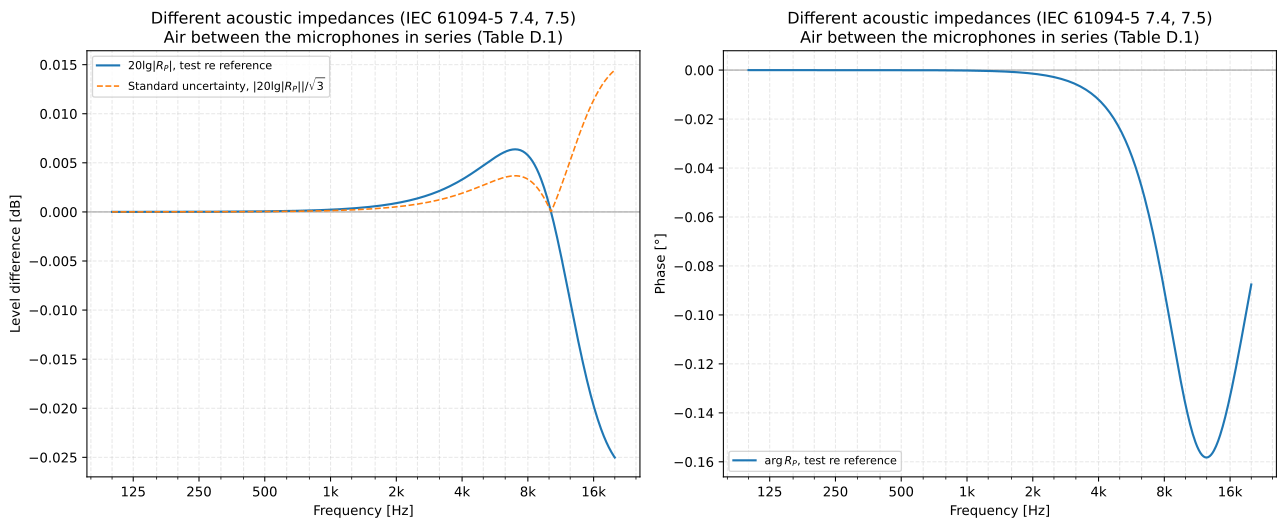
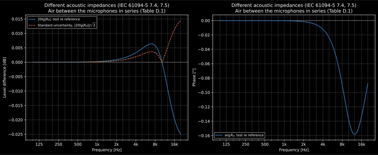
The air between an LS2P and a high sensitivity WS2P in series with each, by the circuit of reference [2]: the level of with its semi-range read as a standard uncertainty (left), and its phase (right).
10. The diffuse-field comparison of IEC 61183
Section titled “10. The diffuse-field comparison of IEC 61183”The diffuse-field method of IEC 61183 clause 5 is a sequential comparison without a monitor: a sound level meter and a reference meter read in turn at the same positions of a reverberation room, the difference of their readings added to the reference’s diffuse-field sensitivity level. The library computes it through the same model, so the two cannot drift apart:
d = metrology.diffuse_field_sensitivity( [1000.0, 2000.0], [94.3, 94.6], [94.0, 94.1], reference_random_incidence_level_db=[-26.0, -26.2],)s = metrology.sequential_comparison([1000.0, 2000.0], [-26.0, -26.2], [94.0, 94.1], [94.3, 94.6])print(d.diffuse_field_level_db, s.sensitivity_level_db) # [-25.7 -25.7] [-25.7 -25.7]11. Validating a jig or a coupler
Section titled “11. Validating a jig or a coupler”“Calibrations performed in any particular jig or coupler shall be validated
by comparison with calibrations performed in other jigs and couplers and
alternative sound sources. A separate validation is necessary for each
different type of microphone. If the test microphone is a laboratory
standard microphone, then the jig or coupler can be validated by comparing
a comparison calibration with a reciprocity calibration. For some
microphones, it can be necessary to use more than one jig and/or coupler to
cover a full frequency range with low uncertainty” (6.7).
metrology.verify_jig_or_coupler sets a calibration made in the jig or
coupler beside another calibration of the same microphone, a comparison made
elsewhere or, for a laboratory standard microphone, the
ReciprocityCalibration of the reciprocity
calibration with the
index of that microphone, and compares them at the frequencies they share.
The clause prints no criterion. The library reads “validated” as the two
agreeing within the expanded uncertainty of their difference, which for two
independent calibrations is the root-sum-square of the two,
Two calibrations that share a component are correlated, and the part they share comes out of (below).
Here the jig of A.2 is validated against the coupler of A.1 for the WS2P of the first example, the coupler used up to the 10 kHz it is for. Near 6,3 kHz the jig has a standing wave close to the microphones, the anomaly Barham et al. found in a test box at that frequency, and the field moves between the reading and the interchange, so (C.3) no longer cancels it:
fv = f[6:] # the jig of A.2, 1 kHz to 20 kHzmode = 0.5 * np.exp(-(((fv / 1000 - 6.3) / 0.6) ** 2)) # the field moves near 6.3 kHzjitter = np.random.default_rng(42).normal(0.0, 0.01, (2, 3, fv.size))j12 = (l_ref[6:] + gain_1) - (l_true[6:] + gain_2) + field_a[6:] + mode + jitter[0]j21 = (l_true[6:] + gain_1) - (l_ref[6:] + gain_2) + field_a[6:] + jitter[1]jig = metrology.simultaneous_comparison(fv, l_ref[6:], j12, j21, expanded_uncertainty_db=u[6:])coupler = metrology.simultaneous_comparison( f[:17], l_ref[:17], l_c12[:, :17], l_c21[:, :17], expanded_uncertainty_db=u[:17]) # the coupler of A.1, up to 10 kHzcheck = metrology.verify_jig_or_coupler(jig, coupler)print(check.passes, check.failing_frequencies_hz.round()) # False [6310.]print(check.unvalidated_frequencies_hz.round()) # [12589. 15849. 19953.]print(check.difference_db[8].round(3), check.expanded_uncertainty_db[8].round(3)) # -0.247 0.128The jig agrees with the coupler at every frequency they share but 6,3 kHz,
where they differ by 0,247 dB against 0,128 dB, and above 10 kHz it is not
validated at all, the coupler not reaching there: a second set-up has to
validate it there, as 6.7 allows. check.normalised_difference is the
difference in units of its expanded uncertainty, -1,93 at 6,3 kHz.
Calibrations that share a reference
Section titled “Calibrations that share a reference”Both calibrations here take the same LS2P as their reference, so the first row of Table D.1, the calibration of that reference (0,025 dB, the “±0,05 dB with a coverage factor of k = 2” of its certificate), is in both budgets. Whatever error that calibration carries moves the two sensitivity levels together and cancels in their difference, while the root-sum-square counts it twice. In the terms of the GUM, two levels that each depend on a common quantity with a sensitivity of 1 have its variance as their covariance (JCGM 100:2008 F.1.2.3, Formula (F.2), whose sensitivity coefficients are then both 1), and the law of propagation for correlated inputs (5.2.2, Formula (13)) gives for the difference
with the standard uncertainty of what the two share.
shared_standard_uncertainty_db takes it, one value or one per frequency of
the calibration, and the band becomes, with the of 7.9,
shared = metrology.verify_jig_or_coupler(jig, coupler, shared_standard_uncertainty_db=0.025)print(shared.passes, shared.failing_frequencies_hz.round()) # False [6310.]print(shared.expanded_uncertainty_db[8].round(3), shared.normalised_difference[8].round(2)) # 0.106 -2.32print(shared.correlation_coefficient[8].round(2)) # 0.31The band narrows from 0,124 dB to 0,101 dB at the low frequencies and from
0,128 dB to 0,106 dB at 6,3 kHz, where the two calibrations are correlated
with a coefficient of 0,31, the reference’s variance over the product of
their standard uncertainties (Formula (14)). The verdict does not change
here: the jig still fails at 6,3 kHz alone, now by 2,32 times the
uncertainty of the difference. A pair that agrees within the root-sum-square
can fail once the shared part is out of it. Which components the two share
is the laboratory’s to say: the calibration of a reference both use, its
drift since then (the row “Drift in reference microphone sensitivity since
last calibration”, 0,017 dB) for two calibrations made close together, a
measuring chain they both go through. Only a component that enters both
levels with the same sign and size belongs here. A reciprocity calibration
made in the same set of three microphones as the reference’s is not such a
case: in IEC 61094-2:2009 Formula (7) (folio 12) the electrical transfer
impedances of the two pairs that go through the third microphone are in the
numerator of one microphone’s sensitivity and in the denominator of the
other’s, so those measurements enter the two levels with opposite signs.
Their covariance is negative and widens the uncertainty of the difference
beyond the root-sum-square, which shared_standard_uncertainty_db cannot
express; only the factors common to both levels with the same sign may be
given there. A shared part larger than either calibration’s standard
uncertainty is refused, since nothing can be shared beyond the whole of it.
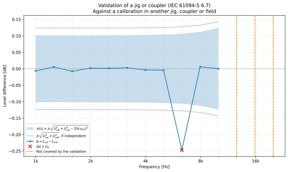
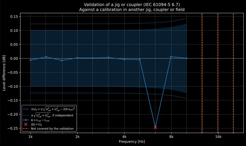
The jig against the coupler: the difference of the two calibrations inside the expanded uncertainty of the difference once the reference they share is taken out, the root-sum-square of two independent calibrations dotted around it, the one frequency where the jig fails, and dashed, the three above 10 kHz the coupler does not reach.
The clause prints neither a criterion nor an example, so the conformance
report checks the verdict against its own definition. Jarvis and Watkins
(1997), NPL Report CIRA(EXT) 022, who compared jig calibrations of working
standard microphones at NPL with reciprocity calibrations of the same
microphones, print no numeric criterion either: their Figures 6 and 7
(folio 4) plot the differences, and the text judges them against “the
typical repeatability” of the measurements (folio 2), one standard
deviation drawn as a band in Figure 7 and never printed as a number, with
no number a criterion could be checked against. The residual differences
“of less than 0.1 dB” of folio 5 report a result rather than set a test, and
the report says nothing about what the two calibrations share. The shared
part has printed numbers, in the GUM: two items
calibrated against the same standard, of relative standard uncertainty
, are correlated with coefficients of about 0,5, 0,990 and 1,000
for comparisons of , and
(F.1.2.3, Example 2). The conformance report checks
correlation_coefficient against them, and the difference of two
calibrations with the budget of Table D.1 against the seven rows left once
the reference’s cancels.
Show the code for these figures
import matplotlib.pyplot as plt
fig, (ax_pressure, ax_free) = plt.subplots(1, 2, figsize=(13.5, 5.6))c.plot(ax_pressure)free.plot(ax_free)fig.tight_layout()
fig, (ax_d1, ax_ff) = plt.subplots(1, 2, figsize=(13.5, 5.6))b.plot(ax_d1)free_field_budget(8000).plot(ax_ff)fig.tight_layout()
fig, ax = plt.subplots(figsize=(10, 6))j.plot(ax)fig.tight_layout()
fig, ax = plt.subplots(figsize=(10, 6))fine.plot(ax, marker="none")ax.plot(j.frequencies_hz, j.correction_db, ls="none", marker="D", label="Table A.1")ax.legend()fig.tight_layout()
fig, ax = plt.subplots(figsize=(10, 6))r.plot(ax)fig.tight_layout()
fig, ax = plt.subplots(figsize=(10, 6))ir_ws2f.plot(ax)fig.tight_layout()
fig, (ax_time, ax_response) = plt.subplots(1, 2, figsize=(13.5, 5.6))ws2f.plot(ax_time)ax_time.set_xlim(1000 * (direct - 0.0015), 1000 * (direct + 0.0035))ws2f.plot(ax_response, quantity="response", frequencies_hz=np.geomspace(1000, 40000, 300))fig.tight_layout()
fig, ax = plt.subplots(figsize=(10, 6))pulse.plot(ax, upper_frequency_hz=20000)fig.tight_layout()
fig, (ax_pressure, ax_free) = plt.subplots(1, 2, figsize=(13.5, 5.6))cp.plot(ax_pressure, quantity="phase")tsel.plot(ax_free, quantity="phase")fig.tight_layout()
fig, (ax_level, ax_phase) = plt.subplots(1, 2, figsize=(13.5, 5.6))rp.plot(ax_level)rp.plot(ax_phase, quantity="phase")fig.tight_layout()
fig, (ax_level, ax_phase) = plt.subplots(1, 2, figsize=(13.5, 5.6))gap.plot(ax_level, marker="none")gap.plot(ax_phase, quantity="phase", marker="none")fig.tight_layout()
fig, ax = plt.subplots(figsize=(10, 6))shared.plot(ax)fig.tight_layout()plt.show()
What this guide covers
Section titled “What this guide covers”Covered
IEC 61094-5:2016 and IEC 61094-8:2012, the calculations: the level model of D.2; the simultaneous excitation with the interchange of Annex C (Formulas (C.1) to (C.3)), required for a pressure calibration, and without it for a free-field one (5.3); the sequential excitation against a monitor microphone (61094-5 5.1.3, 61094-8 A.2); the average over the determinations; the reference’s free-field to pressure difference in a free-field calibration (Table 1, 8.2); the WS3 corrections of Table A.1 with their uncertainty; the budgets of Table D.1 and Table 2 on the GUM with (7.9, D.2, D.3, 8.8), and the combination in linear form D.3 mentions; Tables A.1, D.1, 1 and 2 as published data; and the effective free-field region of Formula (B.1), with the speed of sound of IEC 61094-2 Annex F, and the longest window it allows for a reflection. The phase of the sensitivity (61094-5 5.1.1, 61094-8 5.1) through the interchange and the monitor ratios. IEC 61094-8 Annex B: the time window of B.1.3 (Tukey, Hann, Hamming, and the rectangular one it does not recommend) with the tapered edges of B.1.2, Formula (B.2) through it, the stepped sine of B.2 by Formula (B.3), and the rectangular pulse of the direct impulse method (B.6, Formula (B.10)). IEC 61094-5 7.4 and 7.5: the pressure ratio of microphones of different acoustic impedance in a closed coupler (IEC 61094-2 Formula (3)), with the lumped equivalent volume of IEC 61094-2 E.4 and IEC 61094-1 6.2.2, and in series with the air between two microphones, whose impedance is that of the circuit of Appendix B of the part’s reference [2], Jarvis (1996), with the ratio it prints and the extremes of its graph reproduced. IEC 61094-5 6.5: the correction for a test microphone smaller than its reference by the model of the part’s reference [1], Barham et al. (2014), from any geometry and separation, with its change on doubling the separation that A.2 names; it reproduces every row of Table A.1 from the inputs of the paper’s Table 1. IEC 61094-5 6.7: the comparison of a calibration made in a jig or a coupler with another of the same microphone, by comparison elsewhere or by reciprocity, at the frequencies they share, with the part of their uncertainty the two share taken out of the uncertainty of the difference by the GUM law of propagation for correlated inputs (JCGM 100:2008 5.2.2 and F.1.2.3), whose correlation coefficients of F.1.2.3 Example 2 are reproduced. The IEC 61183 clause 5 comparison computes through the same model. Table D.1 and Table A.1 are reproduced.
Covered, by a reading of the text
The environmental correction. 6.6 and 7.6 ask for the reference to be corrected to the conditions of the test, or the result to the reference conditions, and print no formula; the first-order sum of a coefficient times a deviation for each condition is this library’s reading, with the coefficients the microphone’s own. The mean of the two ratios of 5.1.2 is taken in decibels, as Annex C does. The coverage factor of the WS3 corrections. A.2, the NOTE to Table A.1 and the special case of Table D.1 give their expanded uncertainty as 10 % of each correction without a coverage factor; it is read as the that 7.9 and D.2 report every expanded uncertainty with, so the standard uncertainty is 5 % of the correction. The phase. Neither part prints a phase form of (C.3) or of the monitor ratios; they are the level forms written for the complex ratio that 5.1.1 calls the sensitivity “both modulus and phase”, the half-difference of the interchange taken in one turn. The impedance ratio. 7.4 and 7.5 leave the model to the literature. The coupler is the printed Formula (3) of IEC 61094-2; for a simultaneous excitation the divider, each diaphragm behind the same series impedance from a common source, is the circuit of Appendix B of Jarvis (1996) seen from each microphone, read with the imaginary unit its first microphone’s mass term has lost in the published scan. The standard uncertainty reads the level difference as a semi-range, as that row does; above 10 kHz, for a WS2F against an LS2P, the row asks for it to be established experimentally. The model of 6.5. As printed, the formulas of Barham et al. (2014) with their own inputs do not give their own Table 2; the library reads the radial sensitivity of Formula (4) less 1 and the annulus of Formula (2) from the overall radius, which give it, at a speed of sound the paper does not print. Its uncertainty is the caller’s to estimate: the model gives the change on doubling the separation that A.2 names as approximately the 10 % of Table A.1. The validation of 6.7. The clause prints no criterion, and Jarvis and Watkins (1997), which compared jig calibrations with reciprocity ones, print no numeric one either, judging the differences in words against one standard deviation of repeatability drawn in their Figure 7; agreement within the expanded uncertainty of the difference, the root-sum-square of the two less the part they share, is this library’s reading, and the conformance report checks it against its own definition. Which components two calibrations share is the caller’s to give, and only one that enters both levels with the same sign and size can be given. Formula (B.10) is read as the spectrum of a pulse lasting , as the formula and its first zero say and the text does not.
Not covered
The measurements themselves, and the choice of the set-ups a jig or a coupler is validated against, for each type of microphone (6.7). The sweeps, maximum length sequences and random noise of B.3 to B.5 are
room.impulse_response,room.mls_impulse_responseandelectroacoustics.transfer_function, and the synchronous averaging of B.6.2 issignals.time_synchronous_average, on their own pages; the qualification of the free field by ISO 26101 is on its own page. The values of IEC/TS 61094-7, which are inputs here; the reciprocity calibration of the reference (IEC 61094-2, -3) is the subject of Microphone calibration by reciprocity. The second special case of Table D.1, a microphone calibrated as a system with its preamplifier (0,002 dB, and for the polarising voltage and the capacitance “frequency dependent” and under 0,02 dB above 200 Hz), is not held as data; a budget that needs it takes it throughadditional_components. A covariance that widens the uncertainty of the difference, as between two microphones of the same reciprocity set through the pairs with the third (IEC 61094-2:2009 Formula (7)), is not taken byverify_jig_or_coupler.
References
Section titled “References”- Barham, R., Barrera-Figueroa, S., & Avison, J. E. M. (2014). Secondary pressure calibration of measurement microphones. Metrologia, 51(3), 129-138. https://doi.org/10.1088/0026-1394/51/3/129Reference [1] of IEC 61094-5:2016 and the origin of its Table A.1: the model of Formulas (1) to (5) for microphones of different diameters, with the inputs of Table 1, that diameter_sound_field_correction computes. Formula (4) is read less 1 and the annulus of Formula (2) from the overall radius, the readings that give its Table 2 (an erratum).
- International Electrotechnical Commission. (2000). Measurement microphones – Part 1: Specifications for laboratory standard microphones (IEC 61094-1:2000). 6.2.2 defines the equivalent volume of a microphone from its acoustic impedance, with the ratio of specific heats at the reference conditions taken as 1,40; Table 3 gives the 10 mm³ ± 5 mm³ of an LS2P. Read from BS EN 61094-1:2001, the English text of EN 61094-1:2000.
- International Electrotechnical Commission. (2006). Measurement microphones – Part 7: Values for the difference between free-field and pressure sensitivity levels of laboratory standard microphones (IEC/TS 61094-7:2006). The free-field to pressure sensitivity level difference a pressure-calibrated reference takes in a free-field calibration (IEC 61094-8 Table 1 and 8.2). The values on this page are illustrative, not read from it.
- International Electrotechnical Commission. (2009). Electroacoustics – Measurement microphones – Part 2: Primary method for pressure calibration of laboratory standard microphones by the reciprocity technique (IEC 61094-2:2009). Annex D gives the static pressure and temperature coefficients of laboratory standard microphones in dB/kPa and dB/K, the units the environmental correction takes them in; Annex F is the humid air whose speed of sound sets the free-field region of a time window; Formula (3) is the closed coupler and E.4 the lumped acoustic impedance of a microphone that the impedance ratio is written with.
- International Electrotechnical Commission. (2012). Electroacoustics – Measurement microphones – Part 8: Methods for determining the free-field sensitivity of working standard microphones by comparison (IEC 61094-8:2012). The free-field counterpart: the sequential substitution with a monitor microphone of 5.2 and A.2, the simultaneous excitation of 5.3, the phase of 5.1, the reference calibration options of Table 1, the uncertainty components of Table 2 with the expanded uncertainty of 8.8, and the time-selective processing of Annex B: the effective free-field region of Formula (B.1), the time window of B.1.3, the stepped sine of B.2 (Formulas (B.2) and (B.3)) and the pulse of the direct impulse method of B.6 (Formula (B.10)). Read from BS EN 61094-8:2012, the English text of EN 61094-8:2012, which is IEC 61094-8:2012 unchanged.
- International Electrotechnical Commission. (2016). Electroacoustics – Measurement microphones – Part 5: Methods for pressure calibration of working standard microphones by comparison (IEC 61094-5:2016). The implemented methods: the level model of D.2 and the phase of 5.1.1, the simultaneous excitation with the interchange of 5.1.2 and Annex C (Formulas (C.1) to (C.3)), the sequential excitation with a monitor of 5.1.3 and Annex B, the environmental correction of 6.6, the correction for microphones of different diameters of 6.5 by the model of its reference [1], the validation of a jig or a coupler of 6.7, the effect of different acoustic impedances of 7.4 and 7.5 with the air between two microphones of Table D.1 by the circuit of its reference [2], the WS3 corrections of Table A.1 and the example budget of Table D.1 combined as D.3 asks. Read from Edition 2.0 (2016-05), English-French.
- Jarvis, D. R. (1996). Methods for determining the pressure sensitivity of working standard microphones: a report on Euromet project A311 (NPL Report CIRA(EXT) 010). National Physical Laboratory. Reference [2] of IEC 61094-5:2016: the circuit of Appendix B for the air between two microphones in a symmetric coupler, whose series impedance air_gap_series_impedance_pa_s_m3 gives, and its example of an LS2P against a high sensitivity WS2P. The published scan has lost the imaginary unit of the first microphone's mass term (an erratum).
- Jarvis, D. R., & Watkins, S. (1997). Methods for determining the pressure sensitivity of IEC type WS3 measurement microphones (NPL Report CIRA(EXT) 022). National Physical Laboratory. Jig calibrations of working standard microphones compared with reciprocity calibrations of the same microphones (Figures 6 and 7) and judged in words against the typical repeatability of the measurements, one standard deviation drawn as a band in Figure 7; it prints no numeric criterion for the validation of 6.7, no numbers one could be checked against, and nothing on what the two calibrations share.
- Joint Committee for Guides in Metrology. (2008). Evaluation of measurement data – Guide to the expression of uncertainty in measurement (JCGM 100:2008, the GUM). BIPM. https://doi.org/10.59161/JCGM100-2008EThe law of propagation of uncertainty both budgets are combined by, and the coverage factor k = 2 both parts report with; its form for correlated inputs (5.2.2) with the covariance of two estimates of a common quantity (F.1.2.3) takes what two calibrations share out of the uncertainty of their difference, and the correlation coefficients of F.1.2.3 Example 2 are reproduced. Also published as ISO/IEC Guide 98-3:2008.