A laboratory standard microphone is calibrated without a reference microphone. Two microphones are coupled acoustically, one drives as a sound source and the other receives, and the electrical transfer impedance that is measured is the product of their two sensitivities times the acoustic transfer impedance of whatever couples them, which is computed:
In a coupler (IEC 61094-2) is the acoustic impedance
of a small enclosed volume of gas; in a free field (IEC 61094-3) it is
that of a spherical wave between the two acoustic centres. Three microphones
measured in pairs give three products, and each sensitivity follows from them
alone. The three modules of metrology that do this are
reciprocity_coupler, reciprocity_free_field and reciprocity_calibration,
which holds the result and the budget both share.
The readings on this page are synthetic: electrical transfer impedances built from three sensitivities the page knows, so every step can be checked against them.
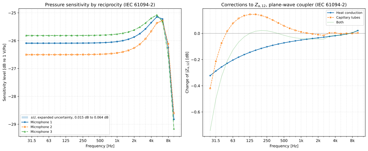
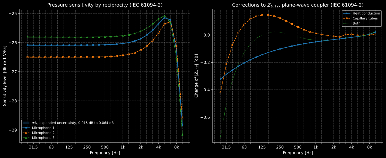
Three LS1P microphones calibrated in a plane-wave coupler (left) and the
corrections to the transfer impedance of one pair (right), from the results’
own .plot().
1. How the measurement goes
Section titled “1. How the measurement goes”Both parts use three microphones, two of which must be reciprocal, or two microphones and an auxiliary sound source, one of which must be reciprocal (5.1.1). Each pair is measured in turn: one microphone is driven by a current, measured as the voltage across a calibrated impedance in series with it, and the other’s open-circuit voltage is read by the insert voltage technique (5.3). The quotient is the electrical transfer impedance. In a coupler the two face each other across a cavity of known shape; in a free field they face each other on their principal axes in an anechoic room.
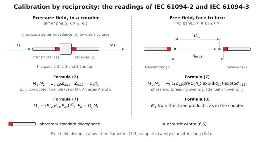
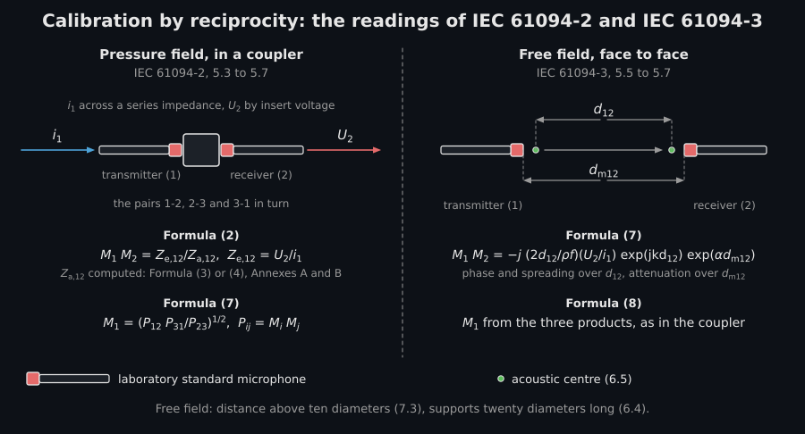
A pair of the triad in a coupler and in a free field: what is measured, what is computed and what each part’s formulas make of them.
| Requirement | Value | Clause |
|---|---|---|
| Reference conditions | 23,0 °C, 101,325 kPa, 50 % relative humidity | 61094-2 and 61094-3, 4 |
| Polarizing voltage | 200,0 V recommended, and the one used reported | 61094-2, 6.2; 61094-3, 6.2 |
| Plane-wave coupler | Distance between the diaphragms 0,5 to 0,75 times the diameter, up to about 10 kHz (LS1P) and 20 kHz (LS2P) | 61094-2, C.2 |
| Large-volume coupler | Length to diameter about 0,3, up to about 2,5 kHz (LS1P) and 5 kHz (LS2P) with a wave-motion correction | 61094-2, C.3 |
| Free-field distance | Greater than ten nominal diameters of the microphone | 61094-3, 7.3 |
| Free-field mounting | On a cylinder of the microphone’s diameter at least twenty diameters long, tapered to its support | 61094-3, 6.4 |
| Reported uncertainty | Expanded, with (61094-2) or for a 95 % coverage probability (61094-3), at each frequency | 61094-2, 7.5; 61094-3, 7.8 |
2. The microphones and the coupler
Section titled “2. The microphones and the coupler”Each microphone enters the acoustic transfer impedance through its acoustic
impedance and its front cavity. Annex E writes the impedance as a lumped
compliance, mass and resistance, or equivalently as the equivalent volume at
low frequencies, the resonance frequency and the loss factor; E.4 states the
representation good to about 1,3 times the resonance frequency. The front
cavity’s measured volume, depth and diameter come from E.2 and E.3. The
coupler is either a plane-wave coupler of the diameter of the front cavities
or a large-volume coupler, with the nominal dimensions of Tables C.1 and C.2
in metrology.IEC61094_2_TABLE_C1 and metrology.IEC61094_2_TABLE_C2.
Figure C.2 draws each microphone of a large-volume coupler with its face a
distance F back from the cavity, through a bore of the front-cavity diameter
B: LargeVolumeCoupler takes that length as port_length_m, and the two
bores of the LS1P coupler add 2,4 % to its volume, a tenth of a decibel on
each sensitivity.
import numpy as npfrom phonometry import fluids, metrology
mics = tuple(    metrology.ReciprocityMicrophone(        equivalent_volume_m3=v,        resonance_frequency_hz=f0,        loss_factor=d,        front_cavity_volume_m3=0.534e-6,   # measured, E.3        front_cavity_depth_m=1.95e-3,      # D of Table C.1        front_cavity_diameter_m=18.6e-3,   # B of Table C.1    )    for v, f0, d in ((148e-9, 8200.0, 1.05), (141e-9, 8350.0, 1.00), (152e-9, 8050.0, 1.10)))coupler = metrology.PlaneWaveCoupler(    length_m=7.5e-3,    diameter_m=18.6e-3,    capillary=metrology.CapillaryTube(length_m=0.05, radius_m=0.2e-3, count=2),)conditions = {"temperature_c": 22.4, "static_pressure_pa": 100200.0, "relative_humidity_percent": 46.0}f = metrology.exact_frequencies(20, 10000, fraction=3)check = metrology.check_coupler(f, coupler, mics, **conditions)print(check.passes, round(check.length_to_diameter_ratio, 3), check.ratio_recommended)   # True 0.613 True
large = metrology.LargeVolumeCoupler(length_m=12.55e-3, diameter_m=42.88e-3, port_length_m=0.80e-3)   # E, C, F of Table C.2print(round(large.cavity_volume_m3 * 1e9), round(large.closed_volume_m3(mics[:2]) * 1e9))   # 18124 19626 (mm³)
check_coupler holds the coupler to what its formulas need: Formulas (A.3)
and (A.4) “are valid for the frequency range given by ”, 3 Hz and 12 Hz for the LS1P and LS2aP couplers of Table C.1; the
approximation (A.2) of a large-volume coupler to and
; and the conditions to the domain Annex F states for its air. Two
things are reported without entering the verdict: the ratio C.2 recommends,
0,5 to 0,75 between the distance of the diaphragms and the diameter, and a
frequency below 20 Hz with the approximation, where A.2 asks for the full
solution “or the corresponding uncertainty component shall be increased
accordingly” (full_solution_advised).
3. The acoustic transfer impedance and its corrections
Section titled “3. The acoustic transfer impedance and its corrections”In the plane-wave coupler, Formula (4) treats the whole system as a transmission line of length between the diaphragms, the coupler plus the two front-cavity depths, terminated at each end by the microphone’s acoustic impedance in parallel with the excess volume of its front cavity (7.3.3.1):
The heat conduction and the viscous losses at the cylindrical wall enter through the propagation coefficient and wave impedance of Formulas (A.3) and (A.4), and the heat conduction at the two diaphragms through the admittance of Formula (A.5). In a large-volume coupler the gas is a pure compliance, Formula (3), and the heat conduction makes its volume look larger by the complex factor of Formula (A.1),
with Gerber’s temperature transfer function of the cylinder and its volume to surface ratio. The capillary tubes that equalise the static pressure shunt the cavity, and Formula (6) divides the transfer impedance by , with the input impedance of an open tube of Formulas (B.1) to (B.3).
pairs = ((0, 1), (1, 2), (2, 0))za = [metrology.coupler_transfer_impedance(f, coupler, mics[i], mics[j], **conditions) for i, j in pairs]print(za[0].heat_conduction_correction_db[[1, 16, 25]].round(3)) # [-0.287 -0.051 0.004]print(za[0].capillary_correction_db[[1, 16, 25]].round(3)) # [-0.213 0.011 -0. ]At 31,6 Hz the heat conduction lowers the transfer impedance by 0,29 dB and
the two tubes by another 0,21 dB; at 1 kHz both are a few hundredths. The two
annexes print tables meant for testing exactly this arithmetic.
temperature_transfer_function sums the full solution of the annex’s
reference [A.1], which A.2 requires below 20 Hz unless the uncertainty
component is increased instead, and which gives every entry of
Table A.1 to the 0,000 01 the annex states for them; Formula (A.2) is the
approximation, accurate to 0,01 % in modulus for :
print(metrology.temperature_transfer_function(1.0, 100.0).round(5)) # (0.97179+0.02758j)print(metrology.temperature_transfer_function(1.0, 100.0, method="approximation").round(5)) # (0.97179+0.02758j)air = fluids.air(temperature_c=23.0, static_pressure_pa=101325.0, relative_humidity_percent=50.0)tube = metrology.capillary_tube_impedance([20.0, 1000.0], length_m=0.05, radius_m=1 / 6000, gas=air)print((tube.impedance_pa_s_m3 / 1e9).round(3)) # [3.015+0.097j 8.331+4.288j]Table B.1 prints 3,015 and 8,331 GPa·s/m³ for this tube, Table B.2 0,097 and 4,287. The radius the table heads “0,1667 mm” is 1/6 mm: with 0,1667 mm the values come out 0,08 % low, beyond the last printed figure (an erratum). Even with 1/6 mm the air of Annex F does not give every entry to its last figure: the 186 complex entries come back within 0,002 GPa·s/m³, the residue reaching 0,0011 in the real part and 0,0018 in the imaginary near the resonances of the tubes, and 0,0005 and 0,0007 from 20 Hz to 250 Hz, as the 4,288 here shows.
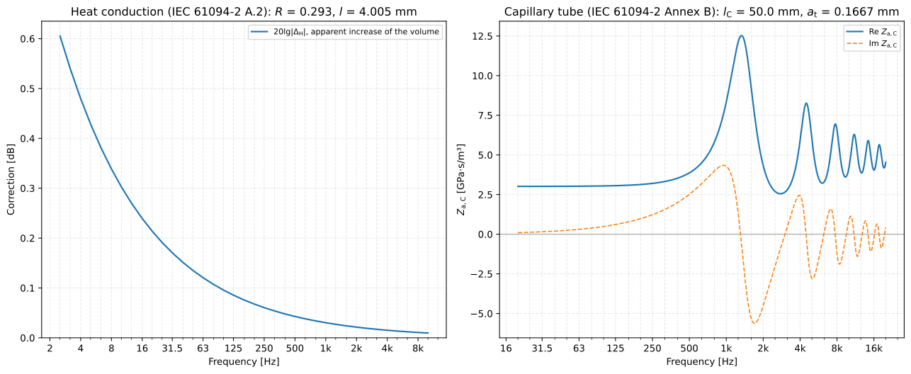
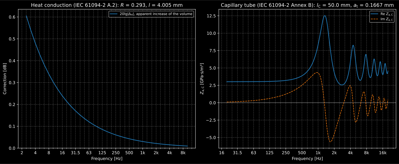
The heat conduction in the large-volume coupler of Table C.2 (left) and the impedance of a capillary tube of Tables B.1 and B.2 at the reference conditions the tables are printed for (right).
Table C.3 prints the wave-motion corrections of the air-filled large-volume coupler for LS1P microphones, to be added to the sensitivity level when they are not determined for the individual coupler; in hydrogen C.3 scales the frequency by the ratio of the speeds of sound:
print(metrology.large_volume_wave_motion_correction([1000.0, 2000.0]).correction_db) # [-0.002 -0.06 ]4. The pressure sensitivities
Section titled “4. The pressure sensitivities”Formula (2) gives the product of each pair, and Formula (7) the three sensitivities from the three products:
true = [m0 * m.complex_equivalent_volume_m3(f) / m.equivalent_volume_m3 for m0, m in zip((0.0496, 0.0473, 0.0512), mics)]ze = [true[i] * true[j] * z.transfer_impedance_pa_s_m3 for (i, j), z in zip(pairs, za)]   # Formula (2)
c = metrology.pressure_reciprocity(f, ze, za)print(c.sensitivity_level_db[:, 16].round(2))    # [-26.03 -26.44 -25.76]print(c.sensitivity_mv_per_pa[:, 16].round(2))   # [49.93 47.64 51.51]print(np.abs(c.sensitivity_v_per_pa - true).max() < 1e-15)   # True
The phase comes from the same products: the complex sensitivity is solved, not
only its modulus. A reciprocity measurement fixes products, and a product does
not change when every sensitivity changes sign together, so the sign of the
square root is a convention. The library takes the branch that is continuous
in frequency with a non-negative real part at the lowest frequency, and
phase_deg refers the phase to 0 to 360° as 5.7.1 of both parts asks. With two
microphones and an auxiliary source, the ratio of their sensitivities measured
against the source replaces the third pair, Formula (8):
pair = metrology.pressure_reciprocity_pair(f, ze[0], za[0], true[0] / true[1])print(pair.sensitivity_level_db[:, 16].round(2)) # [-26.03 -26.44]5. A free-field calibration
Section titled “5. A free-field calibration”In a free field the transmitter is, seen from far enough, a simple source at its acoustic centre. The product of Formula (7) of IEC 61094-3 carries the distance between the acoustic centres, the density of the air, the phase of the spherical wave and its attenuation over the distance the wave travels between the diaphragms:
The attenuation is computed by the five steps of Annex B, ISO 9613-1 adjusted to the quantities of IEC 61094-2, and the wave number takes the speed of sound of IEC 61094-2 Annex F with the dispersion of its NOTE to F.3, which Annex B.1 points to.
ff = metrology.exact_frequencies(1000, 40000, fraction=3)ffc = {"temperature_c": 23.1, "static_pressure_pa": 101100.0, "relative_humidity_percent": 52.0}att = metrology.reciprocity_air_attenuation(ff, **ffc)print(att.attenuation_db_per_m[[0, 10, 13, 15]].round(4)) # [0.0053 0.1348 0.4713 0.9877]Three LS2aP microphones 0,25 m apart, with acoustic centres a few millimetres in front of their diaphragms that recede towards the diaphragm at high frequency (Annex A shows such curves; these are illustrative):
ratio = ff / 23000.0true_ff = [m0 / (1.0 - ratio**2 + 1.3j * ratio) for m0 in (0.0128, 0.0124, 0.0131)]centre = 4.5e-3 / (1.0 + (ff / 30000.0) ** 2)ze_ff = [ metrology.free_field_transfer_impedance( ff, true_ff[i], true_ff[j], diaphragm_distance_m=0.25, acoustic_centres_m=(centre, centre), **ffc ) for i, j in pairs] # Formula (D.1)cf = metrology.free_field_reciprocity( ff, ze_ff, diaphragm_distances_m=(0.25, 0.25, 0.25), acoustic_centres_m=(centre, centre, centre), **ffc)print(cf.sensitivity_level_db[:, 10].round(2)) # [-37.76 -38.03 -37.55]print(np.abs(cf.sensitivity_v_per_pa - true_ff).max() < 1e-15) # TrueFormula (8) as printed omits the factor that it inherits from the three products of Formula (7), and Formula (9), which the corrigendum makes the complex sensitivity, omits it too. The modulus is unaffected; the phase of the printed formulas is 45° off at every frequency, and Formula (D.1) keeps the factor. The library follows Formula (7) (an erratum).
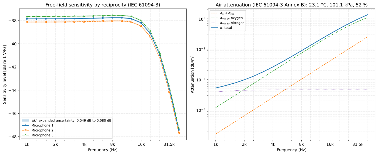
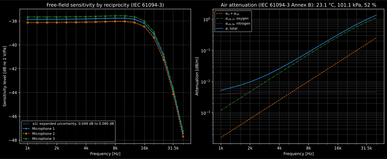
Three LS2aP microphones calibrated in a free field (left) and the attenuation of Annex B (right).
The acoustic centre (6.5). Plotting the inverse of the sound pressure a microphone radiates, corrected for the attenuation, against the distance from a reference point on it gives a straight line in the far field, and where the line crosses the axis is the acoustic centre:
r = np.array([0.15, 0.20, 0.25, 0.30, 0.40, 0.50])alpha = metrology.reciprocity_air_attenuation([10000.0], **ffc).attenuation_np_per_m[0]p = 0.85 * np.exp(-alpha * r) / (r - 2.4e-3) # your readings at one frequencyprint(round(1000 * metrology.acoustic_centre(r, p, attenuation_np_per_m=alpha).position_m, 2)) # 2.4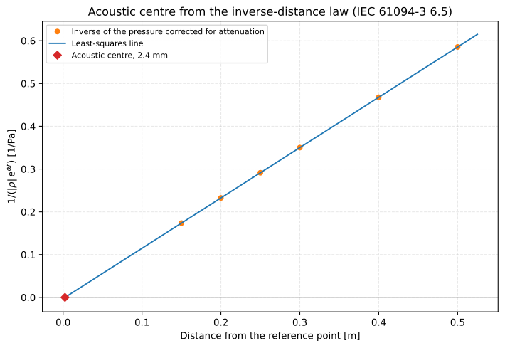
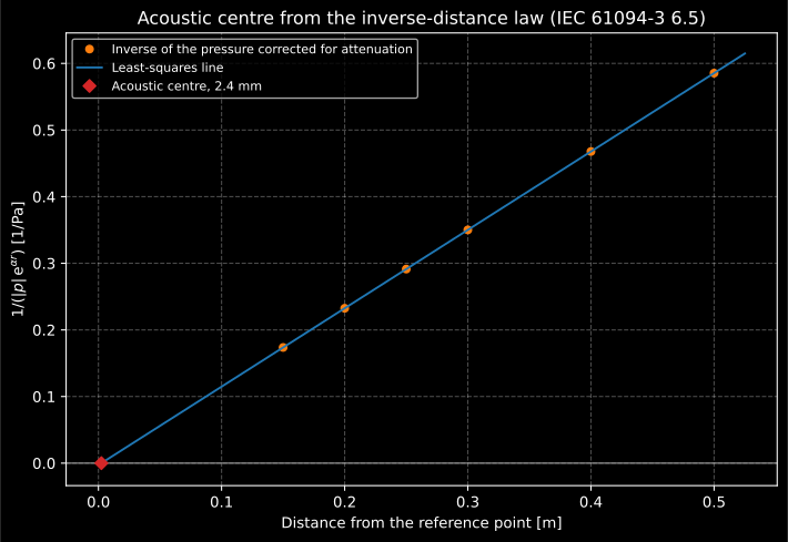
The acoustic centre at 10 kHz: the line through the inverse readings crosses zero 2.4 mm in front of the reference point.
The arrangement. check_free_field_arrangement holds the distance to the
ten nominal diameters 7.3 recommends, the supporting cylinder to the twenty
6.4 recommends and the conditions to the domain in which B.2 states its ±10 %
accuracy: its verdict is whether the arrangement is the recommended one. It
also reports whether the distances are within the 150 mm to 500 mm for which
Annex A gives acoustic centres:
arrangement = metrology.check_free_field_arrangement( ff, diaphragm_distances_m=(0.25, 0.25, 0.25), microphone_diameter_m=13.2e-3, support_length_m=0.3, **ffc)print(arrangement.passes, arrangement.annex_a_range) # True True6. The uncertainty budgets
Section titled “6. The uncertainty budgets”Both parts list the components of a calibration in their Table 1
(IEC61094_2_TABLE_1, IEC61094_3_TABLE_1) and ask for each as a standard
uncertainty as a function of frequency. The components of the acoustic
transfer impedance are found, as both describe, “by repeating a calculation
while the various components are changed one at a time by their associated
uncertainty”: coupler_parameter_uncertainty and
free_field_parameter_uncertainty do that, each microphone’s parameter moved
in turn and the three changes combined into the one row of the table. The
standard uncertainties they move travel together in a
CouplerInputUncertainties or a FreeFieldInputUncertainties, one keyword
per input quantity, and one left at zero adds no component.
pu = metrology.coupler_parameter_uncertainty(    f, coupler, mics,    metrology.CouplerInputUncertainties(        u_coupler_length_m=3e-6, u_coupler_diameter_m=3e-6, u_capillary_radius_m=2e-6,        u_static_pressure_pa=10.0, u_temperature_k=0.05, u_relative_humidity_percent=2.0,        u_front_cavity_depth_m=3e-6, u_front_cavity_volume_m3=1e-9, u_equivalent_volume_m3=1e-9,        u_resonance_frequency_hz=50.0, u_loss_factor=0.03,    ),    **conditions,)print(pu.components_db["capillary_tube_dimensions"][[1, 16]].round(4))   # [0.0086 0.0002]
x = f / 10000b = metrology.reciprocity_uncertainty_budget(    f,    {        **pu.components_db,        "series_impedance": 0.002, "voltage_ratio": 0.003, "cross_talk": 0.001 + 0.004 * x**2,        "polarizing_voltage": 0.0025, "radial_wave_motion": 0.03 * x**2,        "heat_conduction_theory": 0.002, "repeatability": 0.004, "rounding": 0.0006,    },)print(b.expanded_uncertainty_db[[1, 16, 25]].round(3))   # [0.023 0.015 0.041]
pf = metrology.free_field_parameter_uncertainty(    ff,    metrology.FreeFieldInputUncertainties(        u_distance_m=0.1e-3, u_acoustic_centre_m=0.5e-3, u_static_pressure_pa=20.0, u_temperature_k=0.1,        u_relative_humidity_percent=2.0, u_air_attenuation_ratio=0.1 / np.sqrt(3.0),    ),    diaphragm_distances_m=(0.25, 0.25, 0.25), acoustic_centres_m=(centre, centre, centre), **ffc,)xf = ff / 40000bf = metrology.reciprocity_uncertainty_budget(    ff,    {        **pf.components_db,        "series_impedance": 0.002, "voltage_ratio": 0.003, "cross_talk": 0.002 + 0.01 * xf,        "noise": 0.005, "reflections": 0.01 + 0.02 * xf, "polarizing_voltage": 0.0025, "repeatability": 0.01,    },    field="free_field",)print(bf.expanded_uncertainty_db[[0, 10, 15]].round(3))   # [0.049 0.054 0.072]
The expanded uncertainty is times the root-sum-square, which IEC
61094-2 7.5 states; IEC 61094-3 7.8 asks for the factor of a 95 % coverage
probability, which coverage_factor sets when a budget is dominated by a
component with few degrees of freedom. The free-field budget moves each
acoustic centre by 0,5 mm in turn, and the attenuation by the ±10 % B.2
states, taken as a rectangular distribution. The components on this page are
illustrative.
Passed as expanded_uncertainty_db, the budget draws the band of the
calibration’s plot, and its legend states how wide the band is.
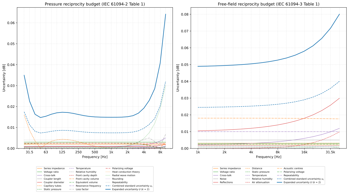
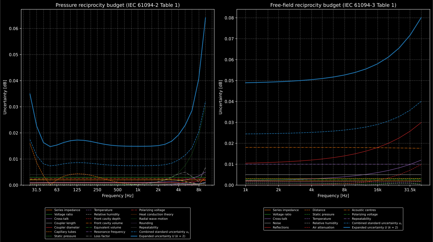
The budgets of microphone 1 of each triad.
Show the code for these figures
import matplotlib.pyplot as plt
# The two calibrations again, with their budgets as the band.c = metrology.pressure_reciprocity(f, ze, za, expanded_uncertainty_db=b.expanded_uncertainty_db)cf = metrology.free_field_reciprocity(    ff, ze_ff, diaphragm_distances_m=(0.25, 0.25, 0.25), acoustic_centres_m=(centre, centre, centre),    expanded_uncertainty_db=bf.expanded_uncertainty_db, **ffc,)
fig, (ax_cal, ax_corr) = plt.subplots(1, 2, figsize=(13.5, 5.6))c.plot(ax_cal)za[0].plot(ax_corr)fig.tight_layout()
fh = metrology.exact_frequencies(1, 10000, fraction=3)heat = metrology.heat_conduction_correction(    fh[fh >= 2.0],    volume_m3=large.closed_volume_m3(mics[:2]),    surface_area_m2=large.closed_surface_m2(mics[:2]),    length_to_diameter_ratio=large.length_m / large.diameter_m,    gas=fluids.air(**conditions),)curve = metrology.capillary_tube_impedance(np.geomspace(20, 20000, 1500), length_m=0.05, radius_m=1 / 6000, gas=air)fig, (ax_heat, ax_tube) = plt.subplots(1, 2, figsize=(13.5, 5.6))heat.plot(ax_heat)curve.plot(ax_tube)fig.tight_layout()
fig, (ax_cal, ax_air) = plt.subplots(1, 2, figsize=(13.5, 5.6))cf.plot(ax_cal)metrology.reciprocity_air_attenuation(metrology.exact_frequencies(1000, 50000, fraction=3), **ffc).plot(ax_air)fig.tight_layout()
fig, (ax_p, ax_f) = plt.subplots(1, 2, figsize=(14.5, 8.2))b.plot(ax_p)bf.plot(ax_f)fig.tight_layout()
fig, ax = plt.subplots(figsize=(7.5, 5.2))metrology.acoustic_centre(r, p, attenuation_np_per_m=alpha).plot(ax)fig.tight_layout()plt.show()
What this guide covers
Section titled “What this guide covers”Covered
IEC 61094-2:2009: the products of Formula (2) and the sensitivities of Formulas (7) and (8), complex; the acoustic transfer impedance of a large-volume coupler by Formula (3) and of a plane-wave coupler by Formula (4), with the excess volume of each front cavity (7.3.3.1), the heat conduction of Annex A (Formula (A.1) with Gerber’s full solution of [A.1] or the approximation (A.2), Formulas (A.3) to (A.5)), and the capillary tubes of Formula (6) and Annex B; the lumped microphone impedance and Formula (E.1) of Annex E; Tables C.1, C.2 and C.3 as published data, the wave-motion correction of Table C.3 with the frequency scaling of C.3 for hydrogen; the check of what the formulas require (A.2, A.3, Annex F); Table 1 and the one-at-a-time recalculation of 7.5. Table A.1 is reproduced to its stated 0,000 01; Tables B.1 and B.2 to within 0,002 GPa·s/m³, more than their printed half-unit near the resonances of the tubes (section 3). IEC 61094-3:2016 with COR1:2016: the products of Formula (7), the sensitivities of Formulas (8) and (9) with the factor of (7), Formula (D.1); the attenuation of Annex B and the speed of sound with the dispersion of IEC 61094-2 F.3; the acoustic centre of 6.5; the arrangement of 6.4 and 7.3; Table 1 and the recalculation of 7.8. Table B.1 is reproduced by ISO 9613-1, as its text says it was computed.
Covered, by a reading of the text
The branch of the square root. IEC 61094-2 asks for the phase “by a similar procedure from the phase angle of each term” and IEC 61094-3 derives it from Formula (8), both referred to 0 to 2π; the library takes the branch continuous in frequency with a non-negative real part at the lowest frequency, and fixes the other two microphones by the products. Dimension F of Table C.2 is the length of the bore that Figure C.2 draws, of the front-cavity diameter B, between each microphone face and the cavity; its volume and its wall join those of the coupler. The surface of a large-volume coupler closed by microphones is that of the closed cylinder plus the wall of each bore, of each front cavity and of its thread, the diaphragm taking the place of the port it closes (7.3.2.2). The ratio of C.2 is read on the distance between the diaphragms, which 5.4 and C.2 call the length of the coupler.
Not covered
The measurements themselves: the insert voltage technique, cross-talk and the ground-shield configuration (5.3, 6.3, 7.2). The radial wave-motion corrections of plane-wave couplers, which C.2 leaves to the literature, and the environmental corrections of Annex D (IEC 61094-2) and Annex C (IEC 61094-3), which are the first-order correction of the comparison guide. The determination of the front cavity and equivalent volumes of E.3 and the data fitting of E.4. The free-field to pressure relation of Formula (4) of IEC 61094-3, which needs the radiation impedance and the scattering factor, and the time-selective processing of Annex D, which follows IEC 61094-8 Annex B. The acoustic centres of Annex A, printed only as a figure.
References
Section titled “References”- International Electrotechnical Commission. (2009). Electroacoustics – Measurement microphones – Part 2: Primary method for pressure calibration of laboratory standard microphones by the reciprocity technique (IEC 61094-2:2009). The pressure calibration: Formulas (2) to (8), the heat conduction of Annex A with Gerber's full solution and the approximation (A.2), the capillary tubes of Annex B, the couplers and wave-motion corrections of Annex C, the microphone parameters of Annex E, Annex F for the air and the uncertainty components of Table 1. Read from BS EN 61094-2:2009, the English text of EN 61094-2:2009, which is IEC 61094-2:2009 unchanged.
- International Electrotechnical Commission. (2016). Electroacoustics – Measurement microphones – Part 3: Primary method for free-field calibration of laboratory standard microphones by the reciprocity technique (IEC 61094-3:2016). The free-field calibration: Formulas (6) to (9) and (D.1), the acoustic centre of 6.5, the arrangement of 6.4 and 7.3, the attenuation of Annex B, Table B.1 and the uncertainty components of Table 1. Read from Edition 2.0 (2016-06), English-French, with its corrigendum IEC 61094-3:2016/COR1:2016 (2016-12), which makes Formula (9) the complex sensitivity.
- International Organization for Standardization. (1993). Acoustics – Attenuation of sound during propagation outdoors – Part 1: Calculation of the absorption of sound by the atmosphere (ISO 9613-1:1993). The method Table B.1 of IEC 61094-3 is computed by, and which B.2 adjusts.
- Joint Committee for Guides in Metrology. (2008). Evaluation of measurement data – Guide to the expression of uncertainty in measurement (JCGM 100:2008, the GUM). BIPM. https://doi.org/10.59161/JCGM100-2008EThe combination both budgets ask for; also published as ISO/IEC Guide 98-3:2008.