Wind turbine sound at a dwelling: IEC TS 61400-11-2
Standards: IEC TS 61400-11ISO 9613
IEC 61400-11 measures what a turbine emits, close to it and downwind. IEC TS 61400-11-2:2024 measures what arrives at a dwelling several hundred metres away, where the wind that drives the rotor also stirs the trees, raises the background and bends the sound on its way. The measurement is long, weeks rather than hours, and everything is sorted by wind speed and direction before it is averaged. This page covers the calculations the TS writes down: the wind speed at the heights the bins need, the bin averages with their uncertainty, the background correction, the low frequency level indoors, the emergence, the amplitude modulation rating and the rating level they feed.
How the measurement goes
Section titled “How the measurement goes”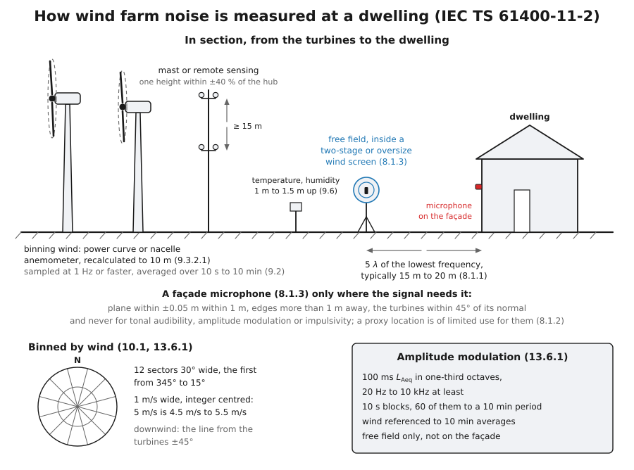
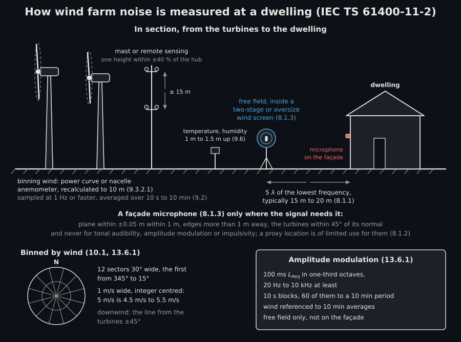
A free-field microphone with a two-stage or oversize wind screen on a tripod or a pole is the preferred mounting (8.1.3). A microphone on the facade raises the signal-to-noise ratio, if the facade is plane within ±0,05 m over 1 m round it and the edges are more than 1 m away, but it cannot be used for tonal audibility, amplitude modulation or impulsivity (8.1.3); a proxy position chosen elsewhere is of limited use for them too (8.1.2). Wind speed and direction come from the turbines themselves, from their power curves or nacelles, or from a mast, and are brought to a 10 m reference height (9.3). Everything acoustic is then binned in 1 m/s wind speed classes and 30° sectors (10.1). For amplitude modulation the sound level meter logs 100 ms in one-third octave bands from 20 Hz to 10 kHz at least, and wind is referenced to 10 min averages (13.6.1).
Wind speed at the heights the bins need
Section titled “Wind speed at the heights the bins need”The power law of Equation (K.1) moves a wind speed between two heights with the shear exponent , and Equation (K.2) inverts it:
Tables K.1 and K.2 evaluate both between 120 m and 10 m. The binning wind speed of 9.3.2 is instead a hub height speed brought down to 10 m with the logarithmic profile and the reference roughness length m of 3.31, which assumes neutral air; the power law through two measured heights carries the stratification with it.
from phonometry import environment
# Table K.1: 8 m/s at 120 m with alpha = 0.3 is 3.8 m/s at 10 m.v10 = environment.power_law_wind_speed(    8.0, height_m=10.0, reference_height_m=120.0, shear_exponent=0.3)# Table K.2: 5 m/s at 10 m under 8 m/s at 120 m is alpha = 0.19.alpha = environment.wind_shear_exponent(    8.0, 5.0, height_m=120.0, reference_height_m=10.0)# The binning wind speed of 9.3.2.1: 8 m/s at the hub, logarithmic, z0 = 0.05 m.v_bin = environment.logarithmic_wind_speed(8.0, height_m=10.0, reference_height_m=120.0)print(round(v10, 2), round(alpha, 2), round(v_bin, 2))   # 3.8 0.19 5.45
profile = environment.wind_shear_profile(4.5, 8.6, upper_height_m=120.0)print(round(profile.shear_exponent, 2), profile.typical)   # 0.26 True
At a wind farm the binning wind speed is the mean of the turbines that make the sound (9.3.2.3). The turbines are sorted by their predicted level at the dwelling and the quietest ones are left out while the total drops by no more than 1 dB; typically two or three remain.
relevant = environment.sound_relevant_turbines( [33.5, 38.2, 29.4, 36.9, 25.1, 31.8, 27.0])print(relevant.indices) # (1, 3, 0)print(round(relevant.total_level_db, 1), round(relevant.relevant_level_db, 1)) # 42.3 41.4print(round(relevant.binning_wind_speed_m_s([6.1, 6.4, 5.8, 6.6, 5.5, 6.0, 5.7]), 2)) # 6.37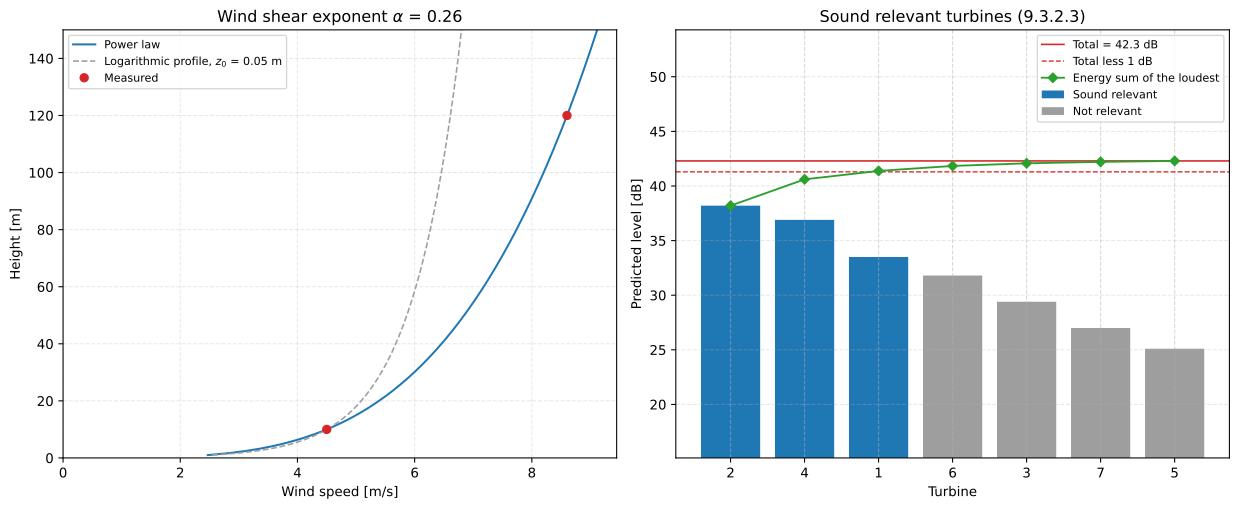
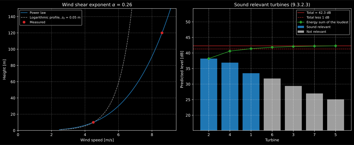
Left: the logarithmic profile of 9.3.2.1 is the neutral atmosphere; on a stable
night the measured shear is larger and the hub sees more wind than the 10 m
speed suggests. Right: leaving out the four quietest turbines drops the total
by 0,9 dB, the fifth would drop it by more, so three turbines set the binning
wind speed; the diamonds are the three loudest together reaching the dashed
line. The figure numbers the turbines from 1, so the indices (1, 3, 0) above
are turbines 2, 4 and 1 on it.
Show the code for this figure
import matplotlib.pyplot as plt
fig, (left, right) = plt.subplots(1, 2, figsize=(13.0, 5.4))profile.plot(left)relevant.plot(right)plt.show()
Bin averages and the background
Section titled “Bin averages and the background”Each bin averages its intervals by energy, Equation (1), or arithmetically for a statistical level such as , Equation (8). The type A uncertainty is the spread about that average over , Equation (2) or (9); the type B part is the root mean square of the per-interval uncertainties, Equations (3) and (4), with examples in Table 3; Equation (5) combines them. The background, measured with the turbines stopped and binned the same way, is subtracted bin by bin under the rule of 11.7: logarithmically, Equation (6) with the uncertainty of Equation (7), where the total is at least 3 dB above it; by a suggested 3 dB where it is at least 0 dB but less than 3 dB above; and not at all where the background is louder, when the turbine level cannot be determined.
import numpy as np
rng = np.random.default_rng(611)speeds = rng.uniform(2.6, 11.45, 420)              # binning wind speeds, m/sturbine = 33.0 + 2.0 * np.minimum(speeds, 9.0)     # rated power at 9 m/sbackground = 15.0 + 3.4 * speeds                   # wind in the treestotal = 10.0 * np.log10(10.0 ** (turbine / 10.0) + 10.0 ** (background / 10.0))total_levels = np.round(total + rng.normal(0.0, 1.2, speeds.size), 1)off_speeds = rng.uniform(2.6, 11.45, 240)           # turbines stoppedoff_levels = np.round(15.0 + 3.4 * off_speeds + rng.normal(0.0, 1.5, 240), 1)
on = environment.bin_sound_levels(total_levels, speeds, type_b_uncertainty_db=0.5)off = environment.bin_sound_levels(off_levels, off_speeds, type_b_uncertainty_db=0.5)corrected = on.background_corrected(off)print(corrected.wind_speeds_m_s)                   # [ 3.  4. ...  10. 11.]print(np.round(corrected.level_differences_db, 1))  # 13.7 ... 3.4 2.1print(np.round(corrected.turbine_levels_db, 1))     # 39.2 ... 50.4 52.2print(corrected.regimes[-1].value)                  # three_db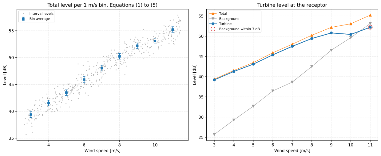
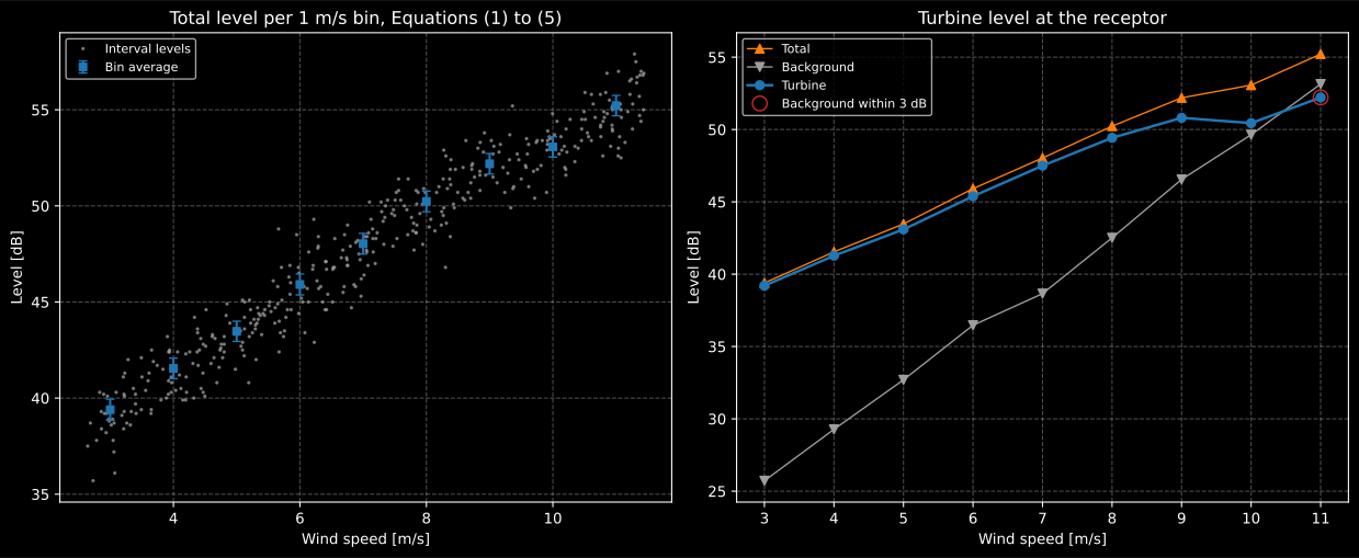
Right: from 3 m/s to 10 m/s the total is 3,4 dB or more above the background and the background is subtracted; at 11 m/s it is 2,1 dB above, and 11.7 suggests taking 3 dB off the total instead. Its NOTE 1 warns that an excess over a limit cannot then be established.
Show the code for this figure
fig, (left, right) = plt.subplots(1, 2, figsize=(13.0, 5.4))on.plot(left)corrected.plot(right)plt.show()A prediction from IEC 61400-11 sound power levels carries its own uncertainty (10.3.4): Equation (10) weights each turbine’s sound power uncertainty by its share of the energy at the dwelling, and Equation (11) adds the 2 dB the TS expects of ISO 9613-2 or Nord2000 downwind and 0,5 dB for the modelling.
prediction = environment.predicted_receptor_level([36.9, 38.2, 33.5], 1.5)print(round(prediction.level_db, 1), round(prediction.combined_uncertainty_db, 2)) # 41.4 2.55Low frequency sound indoors (Annex C)
Section titled “Low frequency sound indoors (Annex C)”Measuring low frequency sound inside a house for weeks is intrusive and rarely clean, so Annex C predicts it from the sound power levels, band by band from 10 Hz to 200 Hz:
with the horizontal distance and the hub height, 11 dB for , the ground correction of Table C.2 for impedance class D, the air absorption and a facade insulation such as the two Danish rows of Table C.3. The turbines are summed per band, and the level is the energy sum of the bands; the Danish limit of C.6.1 is 20 dB for the A-weighted sum from 10 Hz to 160 Hz.
power = 118.0 - np.arange(environment.LOW_FREQUENCY_BANDS_HZ.size, dtype=float)low = environment.wind_turbine_low_frequency_level( np.vstack([power, power, power - 1.0]), # three turbines, 10 Hz to 200 Hz distance_m=[650.0, 820.0, 1100.0], hub_height_m=120.0, facade_insulation_db=environment.LOW_FREQUENCY_FACADE_INSULATION_DB[ "Denmark brick or similar" ],)print(round(low.outdoor_level_db, 1), round(low.indoor_level_db, 1)) # 35.1 16.5danish = environment.LOW_FREQUENCY_BANDS_HZ <= 160.0print(round(10.0 * np.log10(np.sum(10.0 ** (low.indoor_levels_db[danish] / 10.0))), 1)) # 15.8Why Table C.2 sits under ISO 9613-1
Section titled “Why Table C.2 sits under ISO 9613-1”Table C.2’s caption says 70 % relative humidity and 10 °C, and the text under it says the air absorption coefficient is calculated according to ISO 9613-1. From 125 Hz to 200 Hz it is: 0,41, 0,59 and 0,80 dB/km are ISO 9613-1 at that atmosphere, evaluated at the nominal band centres. ISO 9613-1’s own Table 1 is computed at the exact mid-band frequencies and prints 0,584 dB/km (0,58) at 160 Hz, whose exact mid-band is 158,5 Hz; the TS takes nominal centres here, while its Table 7 follows the exact mid-bands. From 50 Hz to 100 Hz it is not. ISO 9613-1 at 70 % gives 0,08, 0,12, 0,19 and 0,28 dB/km at 50 Hz, 63 Hz, 80 Hz and 100 Hz; the table prints 0,07, 0,11, 0,17 and 0,26, which is 0,01 to 0,02 dB/km less.
Those lower cells are not a rounding accident. From 10 Hz to 100 Hz the row is, cell for cell, the air attenuation of the Danish statutory order on wind turbine noise (BEK nr. 135 of 2019, Table 1.4), which is set for 80 % relative humidity and 10 °C, takes the Nord2000 attenuation rates and ignores air absorption below 25 Hz, as the DELTA report behind it recommends. Wetter air absorbs less at these frequencies, and ISO 9613-1 at 80 % gives 0,07, 0,11, 0,17 and 0,25 dB/km there, within 0,01 dB/km of the printed cells. The table therefore joins two atmospheres at 100 Hz: the Danish 80 % below, the caption’s 70 % above. The order stops at 160 Hz with 0,38 and 0,55 dB/km at 125 Hz and 160 Hz, which the TS replaced with its own 70 % values.
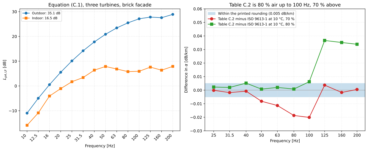
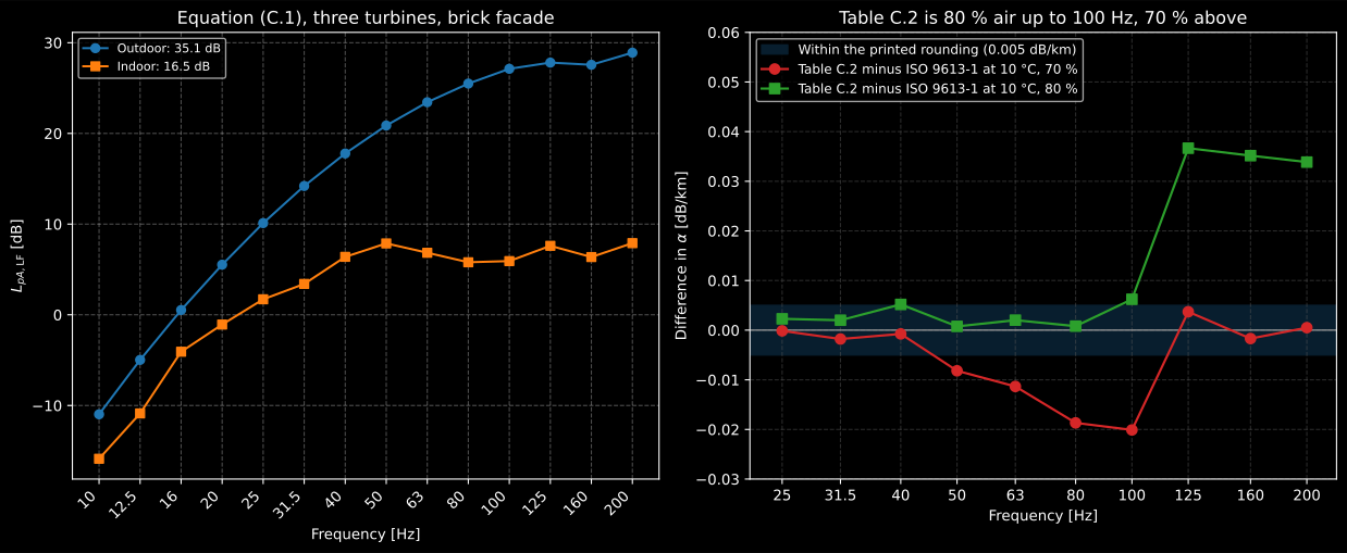
Right: a cell and a computed value that differ by less than 0,005 dB/km print as the same number. Up to 100 Hz the cells are the 80 % atmosphere’s (the 0,006 dB/km at 100 Hz is the Nord2000 band rate of the Danish order, 0,26 where ISO 9613-1 gives 0,254), and from 125 Hz the caption’s 70 % one’s.
Show the code for this figure
import warnings
from phonometry.environment.propagation.air_absorption import air_attenuation
bands = environment.LOW_FREQUENCY_BANDS_HZfig, (left, right) = plt.subplots(1, 2, figsize=(13.0, 5.4))low.plot(left)shown = bands >= 25.0for humidity in (70.0, 80.0):    with warnings.catch_warnings():       # ISO 9613-1 is advisory below 50 Hz        warnings.simplefilter("ignore")        iso = 1000.0 * np.asarray(            air_attenuation(                bands[shown], temperature_c=10.0, relative_humidity_percent=humidity            )        )    printed = environment.LOW_FREQUENCY_AIR_ATTENUATION_DB_PER_KM[shown]    right.semilogx(bands[shown], printed - iso, marker="o",                   label=f"Table C.2 minus ISO 9613-1 at 10 °C, {humidity:.0f} %")right.axhspan(-0.005, 0.005, alpha=0.2)right.set(xlabel="Frequency [Hz]", ylabel="Difference in alpha [dB/km]")right.legend()plt.show()
The difference is at most 0,02 dB/km, a few hundredths of a decibel over the
distances Annex C is used for, but a reader who recomputes the row at the
caption’s atmosphere cannot reproduce its lower half, so it is in the
errata register. The library publishes the row as printed,
LOW_FREQUENCY_AIR_ATTENUATION_DB_PER_KM, and uses it by default, so its
results reproduce the TS and the Danish order; for ISO 9613-1 at another
atmosphere pass the coefficients yourself:
with warnings.catch_warnings(): warnings.simplefilter("ignore") iso_70 = 1000.0 * np.asarray( air_attenuation(bands, temperature_c=10.0, relative_humidity_percent=70.0) )at_70 = environment.wind_turbine_low_frequency_level( np.vstack([power, power, power - 1.0]), distance_m=[650.0, 820.0, 1100.0], hub_height_m=120.0, air_attenuation_db_per_km=iso_70, facade_insulation_db=environment.LOW_FREQUENCY_FACADE_INSULATION_DB[ "Denmark brick or similar" ],)print(round(at_70.indoor_level_db - low.indoor_level_db, 3)) # -0.005Table C.4, the reporting table, adds the distance term that Equation (C.1) subtracts; the equation is the one implemented, and the table is in the errata register.
Emergence (Annex J)
Section titled “Emergence (Annex J)”French regulation limits the emergence, the ambient sound criterion with the turbines running less the background criterion with them stopped, per complete wind speed class, Equation (J.1). It is not a limit on the turbine sound itself.
emergence = environment.sound_emergence( [38.5, 41.0, 43.5], [33.0, 37.5, 41.5], wind_speeds_m_s=[5.0, 6.0, 7.0])print(emergence.emergence_db) # [5.5 3.5 2. ]Amplitude modulation (clause 13)
Section titled “Amplitude modulation (clause 13)”The level of wind turbine sound rises and falls once per blade passage, the “swish” a neighbour describes, and more of it annoys more than its average level says. Clause 13 rates it with the reference method of the Institute of Acoustics Amplitude Modulation Working Group (13.2). The input is a series of 100 ms A-weighted levels summed over seven one-third octave bands, 50 Hz to 200 Hz, 100 Hz to 400 Hz or 200 Hz to 800 Hz (13.6.2.1.1), with three higher bands in Annex G.3 for smaller turbines whose swish lies above 800 Hz.
freqs = [50, 63, 80, 100, 125, 160, 200, 250, 315, 400, 500, 630, 800]rng = np.random.default_rng(7)logged = 40.0 + rng.normal(0.0, 1.0, (1000, len(freqs))) # 100 s, unweighted bandsband_2 = environment.amplitude_modulation_band_levels(logged, freqs, band=2, weighting="Z")print(band_2.shape) # (1000,)One 10 s block (13.6.2.3). The 100 values are de-trended with a cubic fit and transformed with a rectangular DFT of 0,1 Hz resolution into the power spectrum of Equation (12), . The highest local maximum inside the range where the blade passage frequency is expected is the fundamental. Its prominence, Equation (13), is the line over the mean of the two lines beyond each neighbour; a block without a maximum in the range, or with a prominence under 4, is “prominence-failed”. The second and third harmonics join if a maximum sits at, or within one or two lines of, twice and three times the fundamental and both the fundamental alone and the harmonic alone swing more than 1,5 dB. Three lines about each kept component, with their negative frequency mirrors, are transformed back, and the modulation depth is the of that series.
t = np.arange(100) * 0.1rng = np.random.default_rng(1340)levels = np.round( 38.0 + 1.2 * np.sin(2 * np.pi * t / 47.0) # the wind drifting + 2.0 * np.sin(2 * np.pi * 0.8 * t) # the swish, 0.8 Hz + (4.0 / 6.0) * np.sin(4 * np.pi * 0.8 * t + 0.9) # and its harmonic + rng.normal(0.0, 1.0, t.size), 1,)block = environment.amplitude_modulation_block( levels, modulation_frequency_range_hz=(0.5, 1.1))print(block.status.value, block.fundamental_frequency_hz) # valid 0.8print(round(block.prominence, 1), block.harmonic_frequencies_hz) # 79.9 (1.6, 2.5)print(round(block.modulation_depth_db, 2)) # 4.95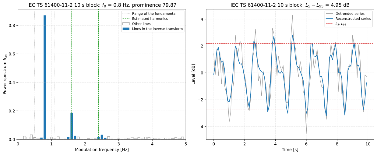
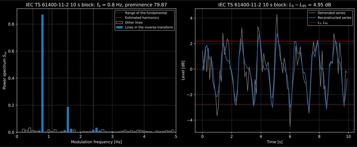
Left: the third harmonic is found at 2,5 Hz, one line above its estimate of 2,4 Hz, which 13.6.2.3 f) allows within two lines. Right: the reconstruction keeps the blade passage and drops the noise.
Show the code for this figure
fig, (left, right) = plt.subplots(1, 2, figsize=(13.0, 5.4))block.plot(left)block.plot(right, kind="series")plt.show()The 10 min rating (13.6.3). Sixty blocks make a period; with at least 30 valid ones, the rating is the 90th percentile of their depths, with the mean and the mode of their fundamentals. A period with fewer is rated 0 dB and gives no modulation frequency. The rating feeds the adjustment of Figure A.1.
t = np.arange(6000) * 0.1rng = np.random.default_rng(1363)depth = 3.0 + 2.5 * np.sin(2.0 * np.pi * t / 600.0) ** 2gust = (t >= 240.0) & (t < 330.0) # 90 s of gusts, no swishdepth[gust] = 0.0series = ( 38.0 + 1.2 * np.sin(2 * np.pi * t / 47.0) + 0.5 * depth * np.sin(2 * np.pi * 0.8 * t) + depth / 6.0 * np.sin(4 * np.pi * 0.8 * t + 0.9) + rng.normal(0.0, 1.0, t.size))series[gust] += rng.normal(0.0, 2.5, int(gust.sum()))period = environment.amplitude_modulation_period( np.round(series, 1), modulation_frequency_range_hz=(0.5, 1.1))print(period.valid_blocks, round(period.rating_db, 2)) # 55 5.84print(round(period.mean_modulation_frequency_hz, 2), period.mode_modulation_frequency_hz) # 0.8 0.8The bins (13.6.4). Each period is a data point of its rating in each band, binned by 1 m/s and 30° like everything else. The mean of each bin counts the 0 dB of the unrated periods and leaves out the excluded ones, and each bin reports the band with the highest mean, with its count, the number of non-zero ratings and the share above 3 dB, 6 dB and 9 dB (13.7).
ratings = np.array( [[2.1, 4.6, 3.0], [0.0, 0.0, 0.0], [1.8, 5.2, 3.9], [2.5, 3.9, 4.4], [0.0, 0.0, 0.0], [3.1, 2.2, 5.0]]) # bands 1, 2 and 3 of six periodsbinned = environment.bin_amplitude_modulation(ratings, [6.2, 6.4, 5.9, 7.1, 7.3, 6.8])print(binned.wind_speeds_m_s, binned.counts) # [6. 7.] [3 3]print(binned.selected_bands, np.round(binned.selected_ratings_db, 2)) # [2 3] [3.27 3.13]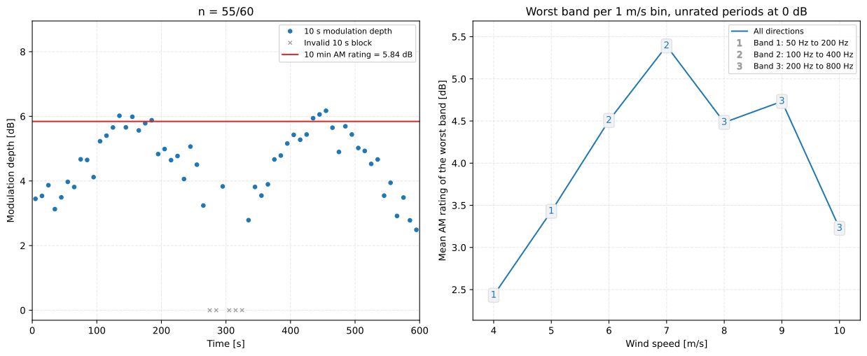
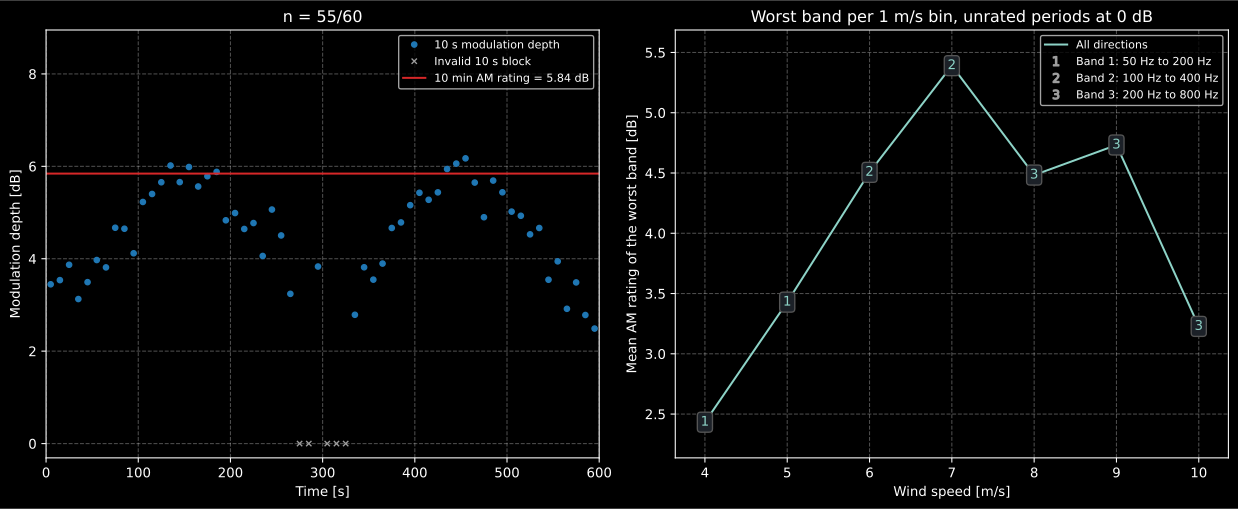
Right: which band carries the swish changes with the wind, and 13.6.4 picks it per bin; the chip over each point names the band, 1 for 50 Hz to 200 Hz, 2 for 100 Hz to 400 Hz and 3 for 200 Hz to 800 Hz. The unrated periods pull the means down where the swish is rare.
Show the code for this figure
rng = np.random.default_rng(1364)survey_speeds = rng.uniform(3.5, 10.45, 600)survey = np.column_stack([ np.clip(1.5 + height * np.exp(-(((survey_speeds - peak) / 2.0) ** 2)) + rng.normal(0.0, 0.8, 600), 0.0, None) for peak, height in ((5.0, 2.5), (7.0, 4.0), (9.0, 4.5))])audible = np.exp(-(((survey_speeds - 7.0) / 2.5) ** 2))survey[rng.uniform(0.0, 1.0, 600) < 0.35 * (1.0 - audible)] = 0.0fig, (left, right) = plt.subplots(1, 2, figsize=(13.0, 5.4))period.plot(left)environment.bin_amplitude_modulation(np.round(survey, 2), survey_speeds).plot(right)plt.show()The TS against the working group’s report and code
Section titled “The TS against the working group’s report and code”Clause 13 says it implements the AMWG Final Report with more specific outputs and the worst case band in each bin, and the 10 s analysis is that report’s step for step. Two differences follow from the TS’s wording, and the TS is what the library implements:
- A period with fewer than 30 valid blocks is rated 0 dB and kept in the
bin mean (13.6.3, 13.6.4); the report discards it (its Figure 4.2.2). 13.6.4
also leaves out “any excluded periods due to pf or other exclusions”. Read
literally, that would drop the very periods 13.6.3 rates 0 dB, whose blocks
failed the prominence test, and the “including 0 values” of the same sentence
and the count of non-zero values it asks for would mean nothing. The library
reads it as the periods the practitioner excludes, the
excluded=flags ofbin_amplitude_modulation. - The band is chosen per bin (13.6.4); the report chooses one band for a whole survey by regressing the bands’ ratings against each other.
A period of exactly 30 valid blocks is rated, as 13.6.2.2 (“at least 50 %”) and the report (“at least 50 % (i.e. 30)”) say; the bullets of 13.6.3 say “greater than” and “less than” and leave it out, which is in the errata register.
The working group published its code (v1.4) with three sample series. It was used here as an oracle and never as a source: the library reproduces the printed sample results, prominence 44.64, fundamental 0.70 Hz and a 10 s rating of 8.38 dB for the 100 Hz to 400 Hz series in the 0.4 Hz to 0.9 Hz range, and agrees with the unmodified code on synthetic blocks and periods, as the conformance report shows. Where the two diverge the TS decides, and the rows pin it: a period of 29 valid blocks is rated 0 dB. One detail belongs to the code alone: it compares the frequencies of its spectrum lines, computed as multiples of 0,1 Hz, with the range limits as floating-point numbers, so an upper limit of 0,6 Hz, 0,7 Hz, 1,2 Hz or 1,4 Hz drops its own line (six, seven, twelve and fourteen times 0,1 Hz come out a little above the limit; sixteen times 0,1 Hz is exactly 1,6 Hz, and that line is kept). The library works in line indices and keeps every limit’s line, as the TS’s “between” reads.
The rating level (Annex A)
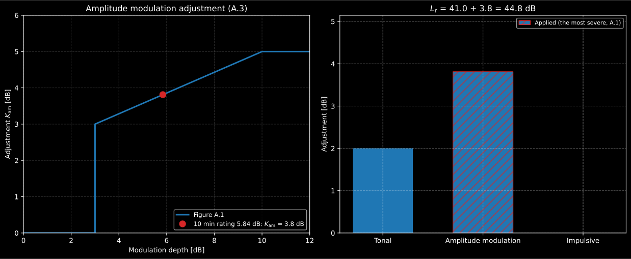
Section titled “The rating level (Annex A)”, with the most severe of the tonal, the
amplitude modulation and the impulsive adjustment, only one at a time (A.1).
The TS’s examples are Table A.1 for tones (ISO 1996-2 Table J.1,
tonal_adjustment_from_mean_audibility),
ISO/PAS 1996-3 for impulses
(impulse_adjustment) and
Figure A.1 for amplitude modulation: nothing below a depth of 3 dB, 3 dB at
3 dB, rising to 5 dB at 10 dB and flat above.
k_am = environment.amplitude_modulation_adjustment(period.rating_db)rating = environment.wind_turbine_rating_level( 41.0, tonal_adjustment_db=2.0, amplitude_modulation_adjustment_db=k_am)print(round(k_am, 2), rating.governing, round(rating.rating_level_db, 1)) # 3.81 amplitude_modulation 44.8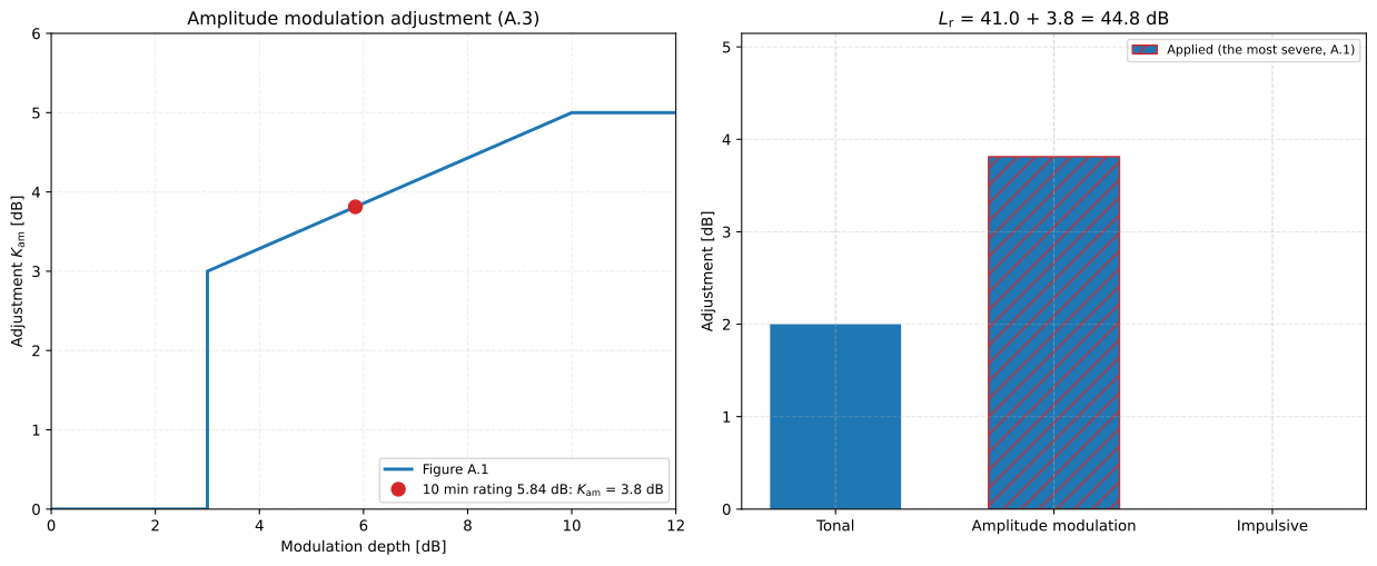
Show the code for this figure
depths = np.linspace(0.0, 12.0, 481)fig, (left, right) = plt.subplots(1, 2, figsize=(13.0, 5.4))left.plot(depths, environment.amplitude_modulation_adjustment(depths))left.plot([period.rating_db], [k_am], "o")left.set(xlabel="Modulation depth [dB]", ylabel=r"Adjustment $K_\mathrm{am}$ [dB]")rating.plot(right)plt.show()Where to stop looking for tones (12.5.2.4)
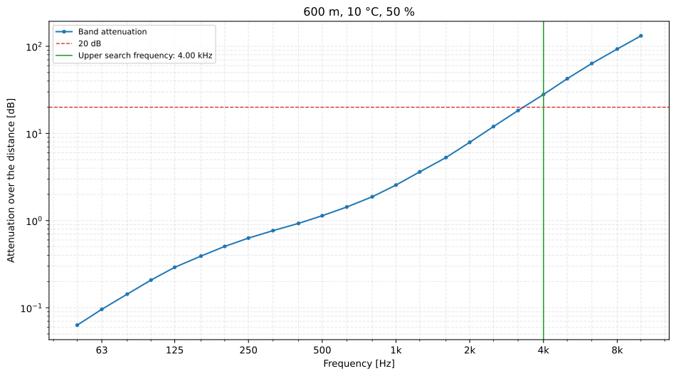
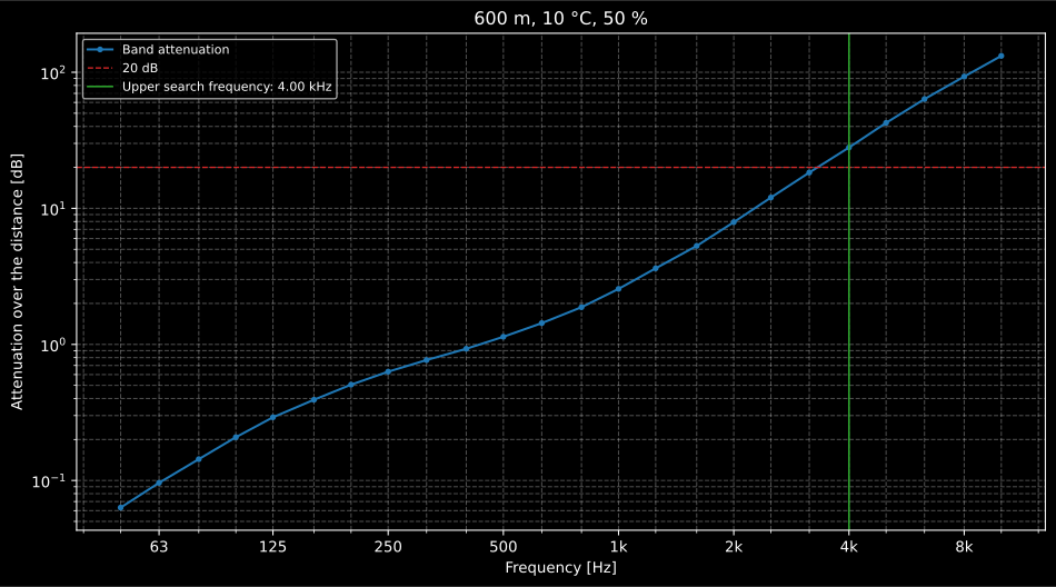
Section titled “Where to stop looking for tones (12.5.2.4)”Tones in a band that ISO 9613-1 attenuates by 20 dB or more over the distance to the nearest turbine are typically of no concern, and every higher band is attenuated more, so the lowest such band sets the top of the search. Table 7 lists it for five atmospheres and four distances; the function computes it for any.
search = environment.upper_tone_search_frequency( 600.0, temperature_c=10.0, relative_humidity_percent=50.0)print(search.upper_frequency_hz) # 4000.0, as Table 7 printsThe row of Table 7 printed for 10 °C and 80 % holds the frequencies the rule gives at −10 °C and 80 % (not those of the table’s own −10 °C row, which is at 100 %); at 10 °C and 80 % the function gives 10, 6,3, 5 and 4 kHz where the table prints 10, 5, 2,5 and 2 kHz. That row, with eight other printed defects of the TS, is in the errata register.
Show the code for this figure
search.plot()plt.show()What this guide covers
Section titled “What this guide covers”Covered
The calculations IEC TS 61400-11-2:2024 writes down: the wind speed between heights of Annex K (Equations (K.1) and (K.2), Tables K.1 to K.3) and the binning wind speed of 9.3.2.1 and 9.3.2.3; the bin averages and uncertainties of Equations (1) to (9) with Table 3, the background correction of Equations (6) and (7) under the rule of 11.7, and the prediction uncertainty of Equations (10) and (11); the low frequency level of Equation (C.1) with Tables C.1 to C.3 and C.5; the emergence of Equation (J.1); the amplitude modulation of clause 13, the 10 s block, the 10 min rating and the bins, with the higher bands of Annex G.3; the rating level of A.1 with the adjustment of Figure A.1; and the upper tone search frequency of 12.5.2.4. Every result plots.
Not covered
The measurement campaign itself: the selection of intervals, the filtering of extraneous sound and the audio auditioning of Annex F are the practitioner’s. The tonal audibility procedure of 12.5 (3 s spectra, the frequency grouping of 12.5.2.6 and the 1 min mean of 12.5.2.7) is not implemented; the library’s tonal audibility is that of ISO/PAS 20065:2016 on the tone audibility page. Nor are the impulsivity of clause 14 beyond the ISO/PAS 1996-3 adjustment, the infrasound of Annex D, the Swedish and Danish criteria as verdicts, or the Nord2000 propagation Annex C builds on. The faster rotors of Annex G.2, whose fundamental modulation frequency lies above 1,6 Hz, are outside it too: the functions refuse a range above the 1,6 Hz of 13.2.
References
Section titled “References”- Institute of Acoustics, Amplitude Modulation Working Group. (2016). A method for rating amplitude modulation in wind turbine noise. Final Report, Version 1, of 9 August 2016: the reference method clause 13 implements, with its 10 s and 10 min methodology. Where the TS departs from it, the TS is followed.
- Institute of Acoustics, Amplitude Modulation Working Group. (2016). IOA AM code. SourceForge. The working group's reference code (v1.4) and its three sample series, the address the TS prints in 13.6.1. Used as an oracle only: the conformance rows reproduce its sample results and its output on synthetic blocks and periods.
- International Electrotechnical Commission. (2024). Wind energy generation systems – Part 11-2: Acoustic noise measurement techniques – Measurement of wind turbine sound characteristics in receptor position (IEC TS 61400-11-2:2024). The implemented edition (Edition 1.0, 2024-03): Annex K and 9.3.2 for the wind speeds, 10.3 and 11.7 for the bins and the background, Annex C for the low frequency level, Annex J, Annex A and 12.5.2.4, and the amplitude modulation of clause 13. Nine of its printed defects are in the errata register.
- International Organization for Standardization. (1993). Acoustics – Attenuation of sound during propagation outdoors – Part 1: Calculation of the absorption of sound by the atmosphere (ISO 9613-1:1993). The air absorption of 12.5.2.4 and of the caption of Table C.2.
- Miljøministeriet. (2019). Bekendtgørelse om støj fra vindmøller (BEK nr. 135 af 07/02/2019). The Danish statutory order whose Table 1.4 is the source of the ground correction, the lightweight facade row and, from 10 Hz to 100 Hz, the air attenuation of Table C.2, set for 10 °C and 80 % relative humidity.