Quality of Outdoor Sound Software (ISO 17534-1)
A noise map is computed by a program, and two programs that implement the same method do not always agree. ISO 17534-1:2015 does not predict a level and does not ask whether a method agrees with measurements; it says how a program shows that it implements its method correctly, and how the user of the program finds out what the program’s shortcuts cost. Two configurations carry the whole standard. In the reference configuration (2.12) every step of the method is performed and none is simplified; in a modified configuration (2.7) one or more steps are approximated, neglected or otherwise simplified, usually to make a large map finish in reasonable time.
Four things in the standard are arithmetic, and
phonometry.environment.propagation.software_quality is those four:
- the comparison of a program’s results with the limits of the certified results of a method’s test cases, which the producer declares in the TRC form of Annex B and the user repeats with every update (7.1);
- the characteristic values and of the level differences between a modified configuration and the reference one (Annex C, 5.2.3, 7.2);
- where the sample of those differences is taken (C.2, C.3);
- the precision of a method across programs, from a round robin (4.5.2, A.3).
The rest (the documentation a method must have, the declaration of conformity, the grade-of-implementation form and the QA data format of Annex D) are requirements on documents.
1. A program against its certified results
Section titled “1. A program against its certified results”A method’s test cases print, for every band and for the total, a correct
result and the interval a program’s result has to fall inside. The final
result is given to two decimal places, and “the result values in frequency
bands and for the total level are considered to be correct if the deviation
does not exceed ±0,05 dB” (Table A.5, note a), which is
CERTIFIED_RESULT_TOLERANCE_DB. A.2 and 4.5.2 put the same rounding interval
another way: the limits are “given to one decimal place”, and “an interval of
0,1 is always included for rounding purposes” when the result ends in 5
(13,65 gives 13,6 to 13,7, which is 13,65 ± 0,05). Table B.2 and every test
case of ISO/TR 17534-3 print the limits to two decimals, which is the
convention the constant follows, and the function compares with whatever
limits it is given. The producer lists each result beside its
limits in the Test Case Results Comparison form (TRC form, Tables B.1 and
B.2) and answers “Result inside tolerances: yes/no”; the user runs the same
cases in the reference configuration “with each new installation or update”
(7.1). verify_calculation_results fills that column. Table B.2, the worked
form for a test case “T XX” of ISO/TR 17534-3, reads:
from phonometry import environment
bands = ["63 Hz", "125 Hz", "250 Hz", "500 Hz", "1 kHz", "2 kHz", "4 kHz", "8 kHz", "Total"]upper = [13.75, 19.55, 21.15, 26.05, 34.85, 37.05, 34.15, 21.65, 40.65]lower = [13.65, 19.45, 21.05, 25.95, 34.75, 36.95, 34.05, 21.55, 40.55]result = [13.7, 19.5, 21.1, 26.0, 34.8, 37.0, 34.1, 21.6, 40.60]
v = environment.verify_calculation_results(result, lower, upper, labels=bands)print(v.passes)                # Trueprint(v.inside)                # (True, True, True, True, True, True, True, True, True)print(v.margins_db.round(2))   # [0.05 0.05 0.05 0.05 0.05 0.05 0.05 0.05 0.05]v.plot()
The verdict is the object: v.passes is the answer, failing_labels names
the rows outside, and bool(v) raises rather than let
if verify_calculation_results(...): pass every program. A limit is part of
the interval, because a deviation that reaches 0,05 dB “does not exceed” it,
and a result that lands on a limit through floating-point arithmetic is on it.
The figure runs the form on this library’s own implementation of ISO 9613-2, with test case T03 of ISO/TR 17534-3 (porous ground, Table 6). The rows are the form’s: the A-weighted level in each octave band and their total, against the row of Table 6, the one its footnote certifies to ±0,05 dB. On the left, the library as it is: every row inside its interval, the largest deviation 0,008 dB. On the right, one detail changed: the air absorption read at the nominal band centres instead of at the exact base-10 midband frequencies of ISO 9613-1, which the attenuation coefficients of ISO 9613-2 are computed at. At 8 kHz that is 8000 Hz instead of 7943 Hz, and it alone moves the band 0,20 dB off its certified result, 0,15 dB below the lower limit, while the total stays inside. This is the kind of implementation detail the form exists to catch, and a total that passes does not show it.
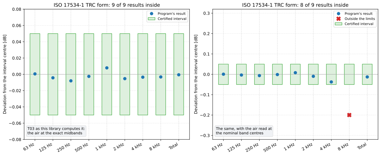
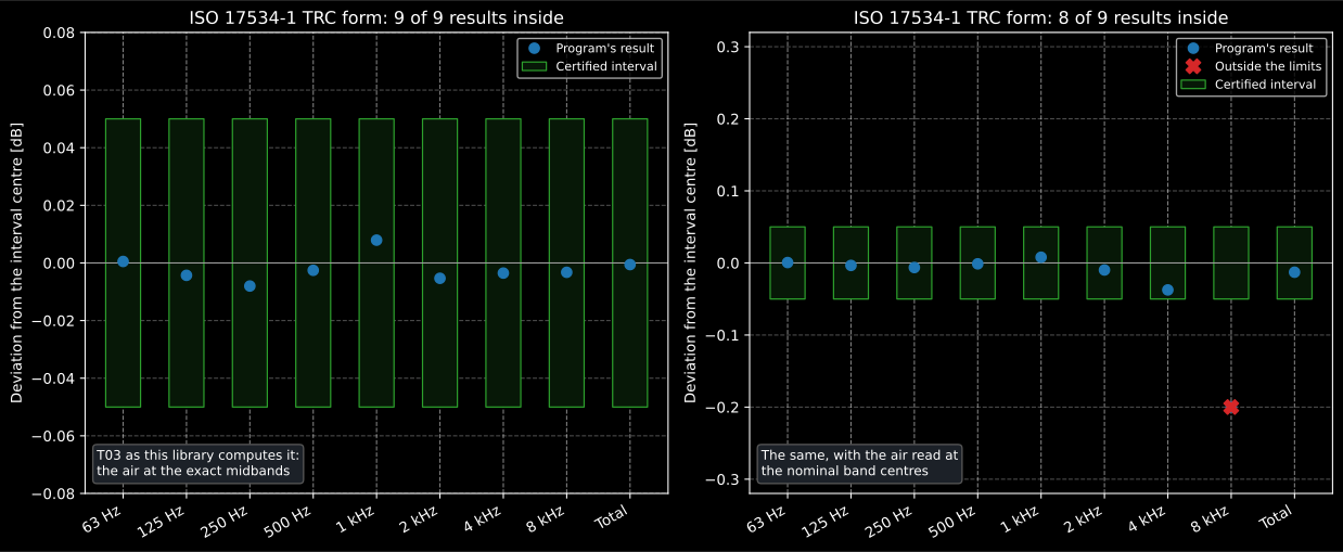
The same test case twice, from the verdict’s own .plot(): the library’s
ISO 9613-2 chain on the left, and on the right with one implementation detail
changed.
Show the code for this figure
import math
import matplotlib.pyplot as pltimport numpy as np
from phonometry import environment
# ISO/TR 17534-3 test case T03: porous ground, 93 dB in every octave, the# source at (10, 10, 1) m and the receiver at (200, 50, 4) m, 20 degC and 70 %.bands = np.array([63.0, 125.0, 250.0, 500.0, 1000.0, 2000.0, 4000.0, 8000.0])d_p = math.hypot(190.0, 40.0)d = math.hypot(d_p, 3.0)levels = np.asarray(    environment.predicted_receiver_level(        np.full(8, 93.0),        environment.PropagationGeometry(d, 1.0, 4.0, projected_distance=d_p),        frequencies=bands,        ground=environment.GroundFactors(1.0, 1.0, 1.0),        atmosphere=environment.AtmosphericConditions(            temperature_c=20.0, relative_humidity_percent=70.0        ),    ))# The same levels with the air absorption read at the nominal band centres.nominal = (    levels    + environment.atmospheric_absorption(        d, frequencies=bands, temperature_c=20.0, relative_humidity_percent=70.0    )    - d * environment.air_attenuation(        bands, temperature_c=20.0, relative_humidity_percent=70.0    ))
# The rows of the form are A-weighted: the eight bands and their total.a_weighting = np.array([-26.2, -16.1, -8.6, -3.2, 0.0, 1.2, 1.0, -1.1])

def trc_rows(band_levels):    weighted = band_levels + a_weighting    return np.append(weighted, 10 * np.log10(np.sum(10 ** (weighted / 10))))

# Row L_A of Table 6 of the report, certified to +/-0,05 dB: bands and total.printed = np.array([13.70, 16.38, 17.73, 23.83, 33.27, 35.69, 32.79, 20.26, 39.14])tol = environment.CERTIFIED_RESULT_TOLERANCE_DBlabels = ["63 Hz", "125 Hz", "250 Hz", "500 Hz", "1 kHz", "2 kHz", "4 kHz", "8 kHz",          "Total"]
fig, axes = plt.subplots(1, 2, figsize=(13, 5.4))for ax, band_levels in zip(axes, (levels, nominal)):    v = environment.verify_calculation_results(        trc_rows(band_levels), printed - tol, printed + tol, labels=labels    )    print(v.passes, v.failing_labels, v.deviations_db.round(3))    v.plot(ax)# True () [ 0.001 -0.004 -0.008 -0.003  0.008 -0.005 -0.004 -0.003 -0.001]# False ('8 kHz',) [ 0.001 -0.003 -0.006 -0.001  0.008 -0.01  -0.037 -0.2   -0.013]plt.show()
2. What a modified configuration costs: the quantiles of Annex C
Section titled “2. What a modified configuration costs: the quantiles of Annex C”A map of a large area is rarely computed in the reference configuration. Programs neglect “the contribution of sources and propagation paths probably not relevant” and interpolate between grid points, and the uncertainties this adds “depend on the individual project” (7.2). So the standard asks every conforming program to let its user measure it (5.2.3): calculate a random sample of receiver points twice, once in the reference configuration and once in the modified configuration the map will really be computed with, and describe the level differences by two order statistics of the sample (Annex C, which is informative). The differences are sorted in ascending order, and the values at two ranking positions are the 0,1-quantile and the 0,9-quantile : 10 % of all the differences in the calculation area are expected below the one and 10 % above the other (C.2, NOTE 2). The two values can go into the legend of the map (7.2).
The standard’s own example sorts 25 differences between two calculation variants and reads , , dB and dB, so that 80 % of the differences are expected between −1 dB and +3 dB:
from phonometry import environment
d = [-1.4, -1.0, -0.4, 0.8, 1.0, 1.0, 1.0, 1.2, 1.4, 1.4, 1.4, 1.6, 1.8,     1.8, 2.0, 2.0, 2.0, 2.2, 2.2, 2.4, 2.6, 2.8, 2.8, 3.0, 3.4]q = environment.level_difference_quantiles(d)print(q.rank_q01, q.rank_q09)                                   # 2 24print(q.q01_db, q.q09_db)                                       # -1.0 3.0print(round(q.mean_db, 2), round(q.standard_deviation_db, 2))   # 1.56 1.17q.plot()
The sample may come in any order; the result keeps it sorted and read-only, and every other value is read from it, so none can disagree with it. C.5 adds two more: the average of the differences, “for considering a systematic deviation”, and their estimated standard deviation, as the uncertainty to carry into an error-propagation calculation by ISO/IEC Guide 98-3. The estimate is the sample standard deviation, with degrees of freedom. The example does not say which variant was subtracted from which. Were the differences the modified configuration minus the reference one, the convention below, the modified configuration would read 1,56 dB high on average, and the quantiles would say more than the mean: a tenth of the area would be expected more than 3 dB high.
Two conventions need saying. A difference is the modified configuration’s level minus the reference configuration’s, so a positive is a shortcut that overestimates. And the quantiles are the statistician’s, not the acoustician’s: C.2 NOTE 2 warns that its leaves 10 % of the values below it, the opposite of a percentile level , which is exceeded 10 % of the time. C.4 says the same thing the other way round: the ranks of are based on and those of on .
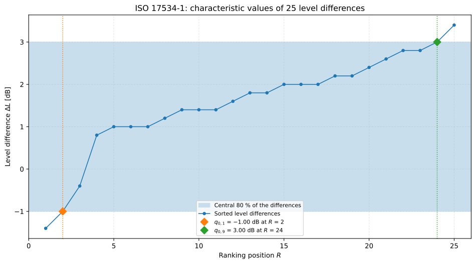
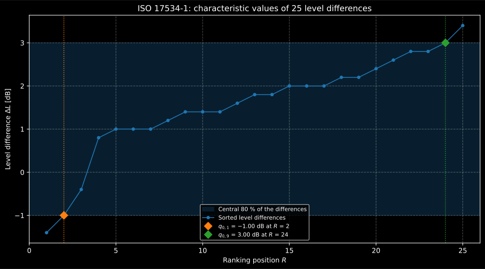
The example of C.4 from the result’s own .plot(): the sorted sample, the
two ranks and the band that holds the central 80 %.
3. Table C.1, the formulas above 50 values, and the seam between them
Section titled “3. Table C.1, the formulas above 50 values, and the seam between them”Table C.1 prints the ranking positions for samples of 20 to 50 values, and above 50 the standard gives two formulas instead,
with IP the integer part (Formulas (C.1) and (C.2)). A sample smaller than 20
is not allowed (C.2). ranking_positions returns the pair, reading
RANKING_POSITIONS, the table as printed, up to 50 values:
from phonometry import environment
for n in (20, 25, 26, 50, 51, 55, 56, 100):    print(n, environment.ranking_positions(n))# 20 (2, 19)# 25 (2, 24)# 26 (3, 24)# 50 (5, 46)# 51 (5, 46)# 55 (5, 50)# 56 (6, 51)# 100 (10, 91)
The table and the formulas do not join. In every one of the 31 rows of the table : it leaves as many values below as above . Formula (C.1) continues the first column and reproduces all 31 rows. Formula (C.2) does not continue the second: it reproduces only 16 of them, and gives one rank less for = 21 to 25, 31 to 35 and 41 to 45. Above 50 it keeps that habit: whenever the last digit of is 1 to 5, leaves one value more above it than leaves below, so at the formula gives 46 where the symmetry of the table would give 47.
| Rule | Values below | Values above | |||
|---|---|---|---|---|---|
| 25 | Table C.1 | 2 | 24 | 1 | 1 |
| 26 | Table C.1 | 3 | 24 | 2 | 2 |
| 50 | Table C.1 | 5 | 46 | 4 | 4 |
| 51 | (C.1), (C.2) | 5 | 46 | 4 | 5 |
| 55 | (C.1), (C.2) | 5 | 50 | 4 | 5 |
| 56 | (C.1), (C.2) | 6 | 51 | 5 | 5 |
The break is in (C.2) alone. Formula (C.1) is the table’s rule carried on, and it is not the rank of the empirical 0,1-quantile (at that rank is 6, and (C.1) gives 5), while (C.2) is exactly that kind of rank, . Written in the shape of (C.2), the symmetric rule would read , and a lost ”+ 5” is conceivable.
Whether it is a slip cannot be settled from the pages that have been read. Annex C was taken from DIN 45687:2006-05, whose Annex F.4 prints the same table, the same two formulas and the same worked example. It bases the ranks of the table on VDI 3723 Blatt 1 (Table 6, column , for , and Table 5, column , for ), and it introduces the formulas with “Falls die Anzahl der Stichproben N > 50 ist, gilt ergänzend zu VDI 3723 Blatt 1 [15] mit ausreichender Übereinstimmung zu E VDI 2450 Blatt 5 [17]”: above 50 values the formulas supplement VDI 3723 Blatt 1, the source of the table, in sufficient agreement with a draft guideline on the quantiles of air-pollutant measurements. ISO 17534-1 dropped both citations, the one in the lead-in of C.4 and the one before the formulas.
VDI 3723 Blatt 1:1993-05 bears the table out and stops where it stops. Its Tables 5 and 6 (printed pages 7 and 8) give the ranking position of the 10 % and the 90 % exceedance levels, and , for samples of up to 50 values, and from 20 to 50 they are the two columns of Table C.1, row for row: the symmetry is already the guideline’s. The guideline goes no further. “Die Werte in den Tabellen 4 bis 6 sind auf n = 50 begrenzt”, it says, since larger samples are hardly ever measured, and for more than 50 values it points to VDI 2450 Blatt 5, then a draft, with no formula of its own (page 7). So the formulas do not come from the source of the table: DIN 45687 brings them in, and only E VDI 2450 Blatt 5, which has not been read here, could say whether (C.2) was meant to follow it rather than the symmetry of the table. A (C.2) that slipped from the symmetric rule in the national standard and travelled into the international one fits the pages that have been read, and so does a (C.2) chosen to agree with E VDI 2450 Blatt 5 while (C.1) kept the table’s rule. So the seam is not recorded as an erratum, and it is not corrected either.
What decides is that ISO 17534-1 and DIN 45687 both print (C.2) this way, and
ranking_positions applies what they print: the table up to 50, the formulas
above. A program that carried the symmetric rule past 50 would report
one rank higher than this one for half of all sample sizes, which is
exactly the disagreement between two quality-assured implementations the
standard is written to prevent. LevelDifferenceQuantiles.from_table says
which of the two rules answered.
4. Where the sample is taken
Section titled “4. Where the sample is taken”The receiver points closer than 2 m horizontally to a source or an obstacle
are left out first (SAMPLE_CLEARANCE_M), and the sample of points is
spread evenly over the that remain: numbered consecutively, the points of
ordinal number , , are taken
(C.2). The standard recommends at least one sample point in a hundred
(RECOMMENDED_SAMPLE_RATIO); a thinner sample is still drawn, with a
SoftwareQualityWarning, because its quantiles are defined, only less
representative of the map.
import numpy as np
from phonometry import environment
print(environment.uniform_sample_indices(2000, 20))# [  50  150  250 ... 1850 1950]
clearance = np.full(2000, 10.0)clearance[:100] = 1.0                      # the first 100 points stand next to a wallprint(environment.uniform_sample_indices(2000, 20, horizontal_clearances_m=clearance))# [ 147  242  337 ... 1857 1952]
print(environment.contour_sample_chainages_m(1234.0, 20))# [  30.   92.  154. ... 1141. 1203.]
The formula leaves two things to the implementer, and both readings are written down in the module. The ordinals are counted from zero: counted from one, the formula would ask for the ordinal 0, which does not exist, whenever is less than , while from zero every sample point sits at the middle of its -th of the list. For a sound contour (C.3), the level of the contour at evenly spaced points is compared with a single-point calculation at the same places, the points sitting at what C.3 calls the “kilometerages” along the contours laid end to end (DIN 45687 F.3: “Kilometrierungen”). A kilometerage is a chainage, a position counted along a route: the word names that position, not the unit it is counted in. Taken in kilometres, the integer part would put every point of a contour shorter than a kilometre at its start, so the chainage is read in metres, and contours so short that two points would fall on the same metre, which can only happen below metres, are refused rather than sampled twice at one place.
5. The precision of a method across programs
Section titled “5. The precision of a method across programs”The same comparison works between programs. With participants of a round robin calculating the same receivers with the same method and the same configuration, the mean at each receiver is the arithmetic mean of the levels, each participant deviates from it by , and “the result of such a round robin test is the quantile according to C.4 of the maximal absolute differences” (4.5.2). The standard’s example is the TestCity scenario of A.3, with four participants and 400 receivers; its Figure A.3 is a histogram of drawn “only shown to demonstrate the principle”, so the figure below builds a synthetic round robin in the same shape.
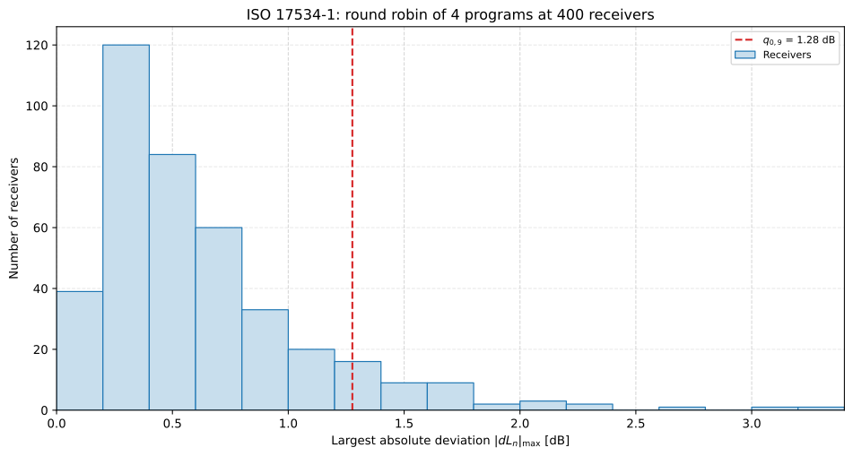
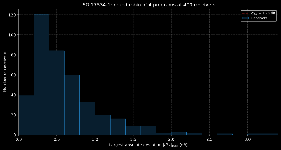
The largest deviation at each receiver, from the result’s own .plot():
nine receivers in ten sit below = 1,28 dB.
Show the code for this figure
import numpy as np
from phonometry import environment
# Four programs at 400 receivers, each off the common level by a spread that# differs from receiver to receiver.rng = np.random.default_rng(17534)common = rng.uniform(45.0, 70.0, 400)spread = 0.15 + 0.6 * rng.gamma(1.5, 0.4, 400)levels = common[:, None] + spread[:, None] * rng.standard_normal((400, 4))
rr = environment.round_robin_precision(levels)print(rr.receivers, rr.participants, rr.rank_q09, round(rr.q09_db, 2))   # 400 4 361 1.28rr.plot()
The mean is arithmetic, not energetic, as the standard defines it, and the quantile is read with the same ranks as Annex C: for 400 receivers, by Formula (C.2).
What this guide covers
Section titled “What this guide covers”Covered
ISO 17534-1:2015, the parts that are arithmetic: the comparison of a program’s results with the limits of the certified results (clause 7.1, the TRC form of Tables B.1 and B.2, the ±0,05 dB of Table A.5, note a), limits included; the ranking positions of Table C.1 and Formulas (C.1) and (C.2) and the characteristic values of C.4, with the mean and the estimated standard deviation of C.5; the uniform sample of C.2 with the 2 m exclusion and the 1:100 recommendation, and the chainages of C.3; and the round-robin result of 4.5.2 and A.3. Table C.1, read also in Tables 5 and 6 of VDI 3723 Blatt 1, the example of C.4 and Table B.2 are reproduced in the conformance report.
Covered, by a reading of the text
Three conventions the text leaves open: the ordinals of C.2 counted from zero, the chainages of C.3 in whole metres, and a level difference taken as the modified configuration minus the reference one. The seam between Table C.1 and Formula (C.2) is applied as printed, for the reasons of section 3.
Not covered
The requirements on documents: the official documentation a method must have (clause 4), the declaration of conformity and the grade-of-implementation form of Annex B, the software properties of 5.2, and the QA data format of Annex D. The programs themselves: nothing here runs a noise map or a modified configuration; the levels to compare come from the program under test. The method-specific test cases are those of ISO/TR 17534-3 for ISO 9613-2, and T08 to T19 of that report, which need barriers, buildings and reflections, are not implemented (see the Outdoor Sound Propagation guide).
References
Section titled “References”- Deutsches Institut für Normung. (2006). Akustik — Software-Erzeugnisse zur Berechnung der Geräuschimmission im Freien — Qualitätsanforderungen und Prüfbestimmungen (DIN 45687:2006-05). The national standard Annex C of ISO 17534-1 was taken from. Its Annex F.4 bases Table C.1 on VDI 3723 Blatt 1 and gives Formulas (C.1) and (C.2) as a supplement to that guideline above 50 values, in sufficient agreement with E VDI 2450 Blatt 5, and it prints (C.2) exactly as ISO 17534-1 does.
- International Organization for Standardization. (1996). Acoustics — Attenuation of sound during propagation outdoors — Part 2: General method of calculation (ISO 9613-2:1996). The calculation method whose implementation the T03 example checks.
- International Organization for Standardization. (2015). Acoustics — Software for the calculation of sound outdoors — Part 1: Quality requirements and quality assurance (ISO 17534-1:2015). The implemented parts: the test-case comparison of clause 7.1 with the TRC form of Annex B (Tables B.1 and B.2) and the ±0,05 dB of Table A.5, note a; the characteristic values of Annex C (C.2 to C.5, Table C.1 and Formulas (C.1) and (C.2)); and the round-robin result of 4.5.2 and A.3. Read from BS ISO 17534-1:2015, whose pages carry the ISO text unchanged.
- International Organization for Standardization. (2015). Acoustics — Software for the calculation of sound outdoors — Part 3: Recommendations for quality assured implementation of ISO 9613-2 in software according to ISO 17534-1 (ISO/TR 17534-3:2015). The method-specific test cases for ISO 9613-2; test case T03 (Table 6, row L_A) is the TRC form worked on this page.
- Verein Deutscher Ingenieure. (1993). Anwendung statistischer Methoden bei der Kennzeichnung schwankender Geräuschimmissionen (VDI 3723 Blatt 1:1993-05). The source DIN 45687 names for Table C.1: its Tables 5 and 6 give the same ranks from 20 to 50 values, symmetric, and it stops at 50 without a formula, pointing to VDI 2450 Blatt 5 for larger samples.