A train passing a microphone is two sources at once: the vehicle, with its wheels, its traction equipment and its bodywork, and the track it runs on, whose rails are rough and whose response to a wheel spreads the vibration along them. ISO 3095 is the type test of rolling stock, the method a vehicle is measured by so that the result says something about the vehicle. It fixes where the microphones stand, what they record and how the runs are averaged, and for the test at constant speed it fixes the track too: a vehicle measured on a rough, lively track is louder than the same vehicle on a smooth, well damped one, and the result is only comparable between sites whose tracks are alike. That second half is two more standards, EN 15610 for the roughness of the rails and EN 15461 for how fast vibration decays along them, and this page covers all three.
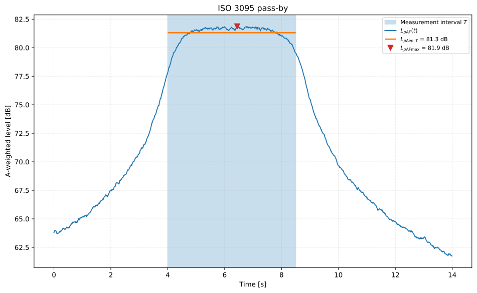
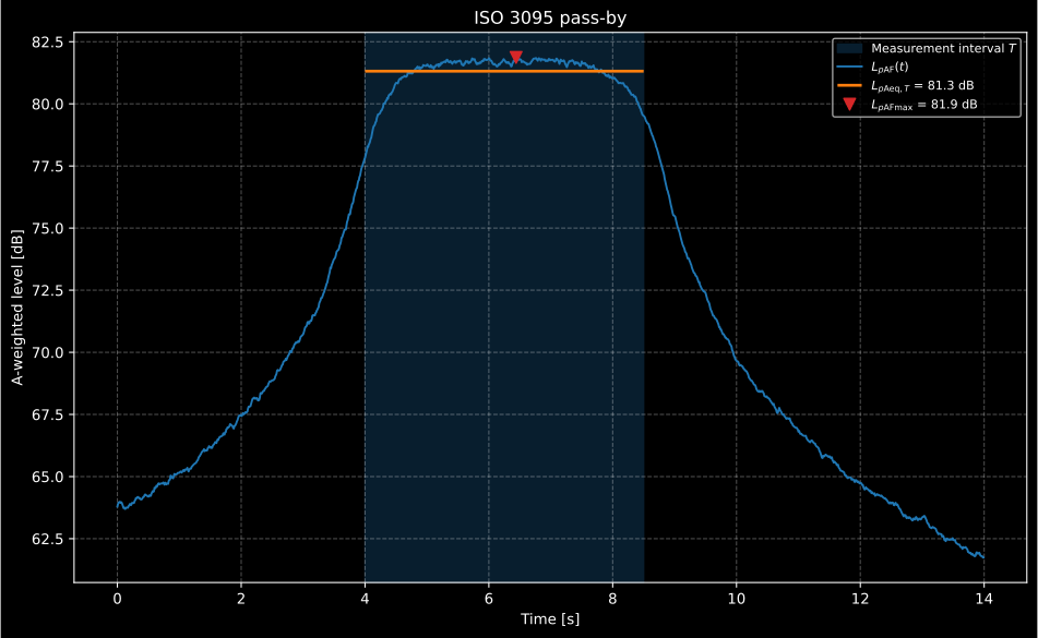
One pass-by: the level history, the interval the unit takes to pass, and the two numbers read from it.
1. Four tests, and the one that needs a track
Section titled “1. Four tests, and the one that needs a track”ISO 3095:2013 has four tests. Each has its own microphone positions and its own measured quantity, and all of them take at least three runs per position, which are valid when they lie within 3 dB of each other (9.3).
| Test | Quantity | Microphones | Result | Clause |
|---|---|---|---|---|
| Stationary | , s | 7,5 m from the track centreline, 1,2 m above the top of rail, at the middle of equal areas 3 m to 5 m long along both sides of every car, plus two at 30° on a 7,5 m half circle off each end of the unit (for a trailer unit, only off the ends with a cab) | The positions energy averaged by the length each stands for, per set; the mean of three sets, rounded to the integer | 5 |
| Constant speed | over the pass-by time | 7,5 m and 1,2 m on both sides; 25 m and 3,5 m allowed at 200 km/h and above | The mean of three runs per side and speed, rounded; the louder side | 6 |
| Starting, maximum level | 7,5 m and 1,2 m, at a cross section 10 m ahead of the unit and along a unit longer than 50 m | The highest of the rounded means | 7.5 | |
| Starting, averaged level | 25 m and 3,5 m, 10 m ahead of the unit | The highest of the rounded means | 7.6 | |
| Braking | , full service braking from 30 km/h | 7,5 m and 1,2 m, opposite the middle of the first car at standstill, ±10 m | The highest of the rounded means | 8 |
Only the constant-speed test needs a reference track. The starting and braking tests ask for a track without joints or visible defects (7.3, 8.2), but only at constant speed does the rolling noise the track shares in dominate the result, and only there does the standard limit the rail roughness and the decay rates (6.2), both printed as numbers. A vehicle can still be measured on a track that misses either limit, but its result then belongs to that site.
How the measurement goes
Section titled “How the measurement goes”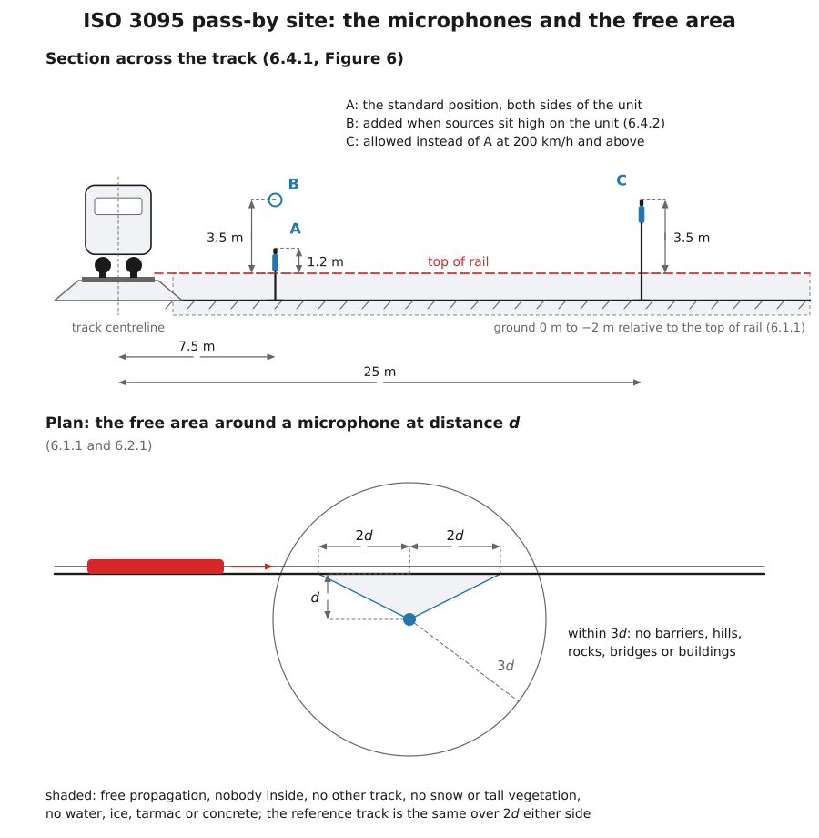
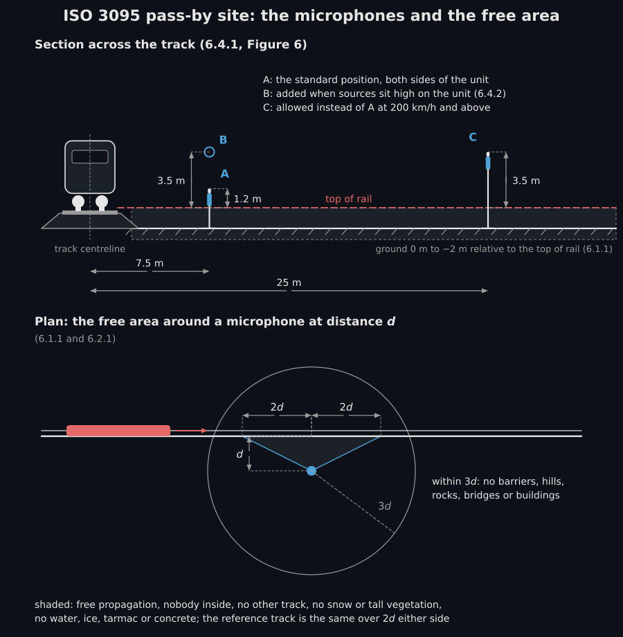
The microphones of the constant-speed test and the area around them that has to be free.
| Requirement | Value | Clause |
|---|---|---|
| Microphone | 7,5 m from the track centreline, 1,2 m above the top of rail, both sides of the unit (one side is enough when the two are acoustically identical); 25 m and 3,5 m allowed from 200 km/h; 7,5 m and 3,5 m recommended as well when there are sources high on the unit | 6.4.1, 6.4.2 |
| Free propagation | Over the triangle between the track and the microphone, reaching twice the microphone distance along the track either side: the ground 0 m to −2 m from the top of rail, no other track, no snow or tall vegetation, no water, ice, tarmac or concrete, nobody inside | 6.1.1 |
| Reflecting objects | None large within three times the measurement distance of the microphone | 6.1.1 |
| Background | over 20 s of background at least 10 dB under the pass-by level, in every band of interest when spectra are asked for | 6.1.3 |
| Speed | Held within ±5 % over the measurement section, measured with a maximum permissible error of 3 % | 6.6.2 |
| Record | Starting at least 10 dB below the level when the front of the train is opposite the microphone and ending 10 dB below the level when the rear is | 6.6.3 |
| Track | A consistent superstructure over twice the microphone distance either side; ballast, wooden or concrete sleepers, no shielding; no joints or visible defects; the roughness and decay-rate limits of 6.2.5 and 6.2.6; a curve radius of 1 000 m, 3 000 m or 5 000 m depending on the speed, and a gradient of at most 5:1 000 where powered units are tested | 6.2 |
2. The pass-by level and the transit exposure level
Section titled “2. The pass-by level and the transit exposure level”The quantity of the constant-speed test is the A-weighted equivalent level over a measurement interval from to (3.14),
and for a multiple unit or a fixed formation the interval is the pass-by time
of the whole unit, from its front to its rear, (6.6.3). Inside a
train the interval runs from the centre of the first unit under test to the
centre of the last. pass_by_measurement A-weights a pressure record, keeps
the level history with time weighting F, and reads the
equivalent level and the maximum within the interval it is given:
import numpy as npfrom phonometry import environment
fs = 16000length_m, speed_kmh, distance_m = 100.0, 80.0, 7.5tp = environment.pass_by_time(length_m, speed_kmh=speed_kmh)t = np.arange(int(14.0 * fs)) / fsfront_s = 4.0                                  # the front passes the microphone at 4 sx_front = speed_kmh / 3.6 * (t - front_s)      # metres the front is past the microphone# The unit as an incoherent line source of its own length: the mean square at# the microphone follows the angle the unit subtends there.angle = np.arctan(x_front / distance_m) - np.arctan((x_front - length_m) / distance_m)rng = np.random.default_rng(3095)p = 0.25 * np.sqrt(angle / np.pi + 1e-4) * rng.standard_normal(t.size)
passby = environment.pass_by_measurement(p, fs, start_s=front_s, end_s=front_s + tp)print(round(tp, 2), round(passby.equivalent_level_db, 1), round(passby.max_level_db, 1))# 4.5 81.3 81.9   T_p in s, L_pAeq,Tp and L_pAFmax in dB
6.6.3 also asks that the record itself start at least 10 dB below the level when the front is opposite the microphone and end 10 dB below the level when the rear is. Given when the front and the rear pass, the result keeps both margins and says whether they are enough.
The 2005 edition of the standard defined one more quantity, the transit exposure level: the energy of the whole passage, measured over an interval long enough to hold all of it, spread over the pass-by time alone (ISO 3095:2005, 3.14, Formulae 8 to 10),
The 2013 edition dropped it, but it is still quoted, and its form survives in
Formula B.1, where a single trailer at the end of a train is measured from its
centre onwards and the energy spread over the pass-by time of half the unit.
Pass the pass-by time to pass_by_measurement and the result carries the
energy of its interval spread over it:
whole = environment.pass_by_measurement( p, fs, start_s=0.0, end_s=14.0, pass_by_time_s=tp, front_passing_s=front_s, rear_passing_s=front_s + tp,)print(round(whole.start_margin_db, 1), round(whole.end_margin_db, 1), whole.recording_interval_sufficient)# 14.0 17.8 Trueprint(round(whole.equivalent_level_db, 1), round(whole.normalized_level_db, 1))# 77.1 82.0 L_pAeq,T over the whole 14 s record, and TELThe transit exposure level is 0,7 dB above the pass-by level here because it
also counts the energy of the approach and the departure, which the pass-by
level leaves out. transit_exposure_level is Formula 10 on its own, for a
level and two durations already known.
3. Three runs, a rounded mean and the louder side
Section titled “3. Three runs, a rounded mean and the louder side”Every test ends the same way: the runs of each position are averaged
arithmetically, the mean is rounded to the nearest integer decibel, and the
result is the highest of those means, the louder side at constant speed and
the loudest position when starting or braking (6.7.1, 7.5.4, 7.6.4, 8.7).
rolling_stock_test does it for any of the four methods, and says whether the
runs of every position lie within the 3 dB of 9.3:
test = environment.rolling_stock_test( {"left": [81.3, 82.1, 81.6], "right": [80.4, 80.9, 81.2]})print(dict(test.reported_levels_db), test.final_level_db, test.valid)# {'left': 82.0, 'right': 81.0} 82.0 TrueThe standard rounds to the nearest integer without a rule for a value that falls on the half; the library rounds a half up, and says so in the result’s documentation. A speed normalisation, where one is asked for, goes on the runs before this (6.7.1).
The clauses around the test are small rules the library states as functions: the type-test speeds of 6.6.2, 80 km/h and the maximum speed or the maximum alone up to 80 km/h; the smallest curve radius of 6.2.2; and the positions of the maximum level starting test, 10 m ahead of the unit, 10 m ahead of its middle when it is longer than 50 m, and evenly between them when those two are more than 50 m apart (7.5.1.1, Figure 10):
print(environment.type_test_speeds(160.0), environment.minimum_curve_radius(160.0))# (80.0, 160.0) 5000.0print(environment.acceleration_test_positions(108.0))# [-10. 17. 44.] metres behind the front of the unit, as Figure 10 draws themThe stationary test averages the positions of a set on energy, weighting each by the length of the unit it stands for, m for the positions off the ends (5.8.1, Formulae 1 and 2), and reports the mean of three sets rounded to the integer:
# A 20 m locomotive: four 5 m areas a side, and two positions off each end.side = [66.0, 68.5, 70.0, 67.0]ends = [64.0, 63.5]mesh = np.array(side + side + ends + ends)sets = mesh + np.array([[0.0], [0.4], [-0.3]]) # three sets, one row eachlengths = [5.0] * 8 + [environment.STATIONARY_END_POSITION_LENGTH_M] * 4standing = environment.stationary_test(sets, lengths)print(standing.set_levels_db.round(2), standing.reported_level_db)# [66.31 66.71 66.01] 66.04. The reference track
Section titled “4. The reference track”4.1 The roughness of the rails (EN 15610)
Section titled “4.1 The roughness of the rails (EN 15610)”A rail’s acoustic roughness is the height of its running surface along it, measured with a probe on a line along the rail head (EN 15610, 3.1). The record is processed in three stages before its spectrum is taken (7.1). The joints, welds and defects are edited out by the operator. Narrow upward spikes, from grains of dirt under the probe, are removed: a spike is where the second derivative falls below and the first derivative changes sign, its edges are where the slope falls below , and it is replaced by a straight line when its height is more than with m, so a narrow peak goes and a broad one, which a wheel does feel, stays (7.2). Every point is then raised to where a wheel of 0,375 m radius would rest on it, because the probe reaches into pits a wheel rolls over (7.3).
Method A of 7.4.2 then cuts the record into segments at least 1 m long overlapping by half, removes the trend of each, applies a Hanning window and averages their spectra; the one-third octave band value is the energy of the lines inside the band, the two lines that straddle an edge counted for the part of their width inside it (Annex C). The level is dB with (3.3), and a segment resolves wavelengths up to a quarter of its length (7.5), so a 1 m segment reports from the 0,25 m band down.
limit = environment.REFERENCE_TRACK_ROUGHNESS_LIMIT_DBx = np.arange(0.0, 20.0, 1.0e-3)               # 20 m of rail, one sample per millimetre
def rail(offsets_db, seed):    """A record whose bands sit 3 dB under the limit, or where offsets_db says."""    rng = np.random.default_rng(seed)    r = np.zeros_like(x)    for wavelength, level in limit.items():        target = level + offsets_db.get(wavelength, -3.0)        k = 10.0 ** np.linspace(-0.045, 0.045, 10) / wavelength  # ten lines across the band        amplitude = np.sqrt(2.0 * 10.0 ** (target / 10.0) / k.size)        for kk in k:            r += amplitude * np.cos(2.0 * np.pi * kk * x + rng.uniform(0.0, 2.0 * np.pi))    return r
# Rail 1 a little corrugated from 5 cm to 2,5 cm, rail 2 at 4 cm and 3,15 cm.left = rail({0.05: -1.0, 0.04: 2.0, 0.0315: 2.5, 0.025: 0.5}, seed=1)right = rail({0.04: 1.0, 0.0315: 1.5}, seed=2)left[7300] += 25.0                             # a grain of dirt under the probespectra = [    environment.acoustic_roughness_spectrum(r, sample_spacing_m=1.0e-3)    for r in (left, right)]print(spectra[0].segment_count, spectra[0].wavelengths_m[0], spectra[0].wavelengths_m[-1])# 39 0.25 0.0025print(round(spectra[0].level_at(0.0315), 1), round(spectra[1].level_at(0.0315), 1), limit[0.0315])# -2.6 -3.6 -5.0   dB re 1 um: both rails over the limit in the 3,15 cm band
The limit is ISO 3095’s Figure 2, and the figure prints its value beside
every point, twenty-two of them from 0,4 m to 3,15 mm, so the library reads
the numbers rather than a curve (REFERENCE_TRACK_ROUGHNESS_LIMIT_DB). The
Annex B listing of EN 15610 types the same twenty-two values as its “2007 TSI
limit”, a second printing the conformance suite checks the first against. Up
to 190 km/h the roughness has to be known from 0,003 m to 0,10 m, and above
it to 0,25 m (6.2.5). The spectra of the records of one line are averaged on
their mean squares (average_roughness_spectra, 7.6), and 6.4.3 sets how
many lines a rail is measured on by the width of its running band
(roughness_measurement_lines).
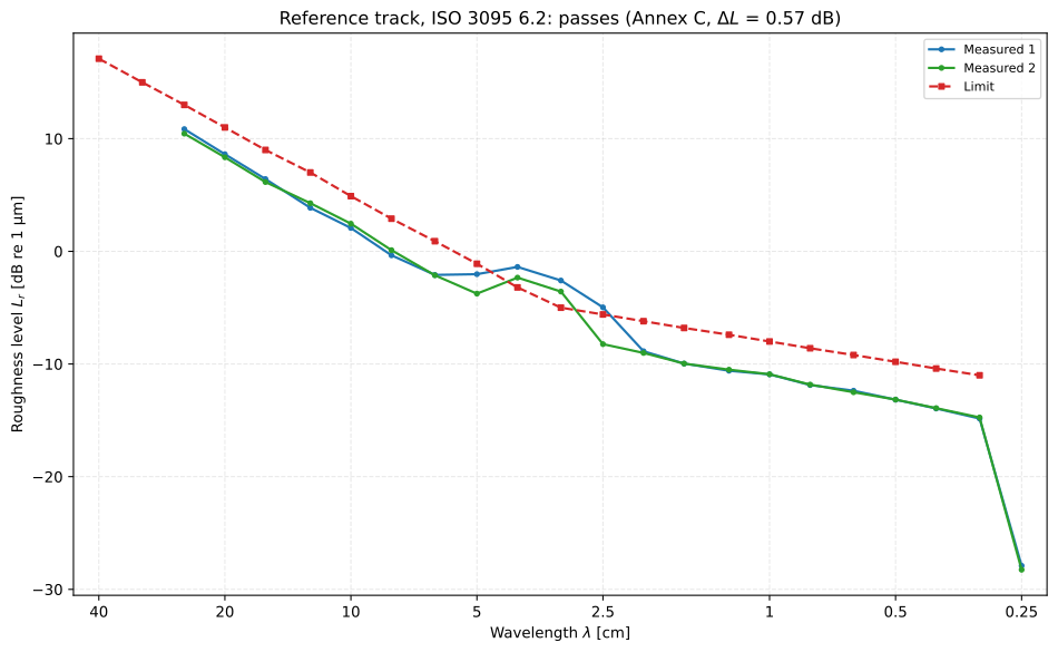
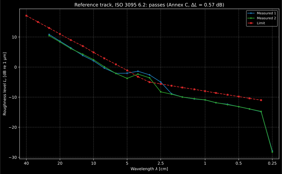
The two rails against the limit of Figure 2: under it everywhere but at 4 cm and 3,15 cm, where both exceed it, and at 2,5 cm, where one does. The track passes only through Annex C (section 4.4), and the title says so.
Method B, filters along the rail (7.4.3). The other way to the same
spectrum runs the processed record through digital one-third octave band
filters and takes the mean square of what comes out of each. A filter starts
from rest at the head of the record and rings for a while, so 2 m of every
output are discarded at either end; a record needs 5 m to leave the 1 m a
spectrum needs (NOTE 1), and the records of one line need at least 15 m
analysed in total once those ends are gone. The filters “shall comply with
EN 61260”, the 1995 edition EN 15610 dates in its references. The bank here
is the library’s own filters.OctaveFilterBank, run at the record’s samples
per metre, so that its frequencies are wavenumbers and its bands are the
base-ten bands Method A reports (roughness_filter_bank). Graded by
filters.verify_filter_class against that edition, it is class 0, the
tightest, and its integrated response (4.5.3) and the sum of its outputs
(4.9) are within class 0 as well. Every band runs at the record’s own rate,
without the band-by-band decimation the library’s banks use by default.
4.8 asks the anti-alias filters of a sampled-data system to keep the
wavenumbers that fold onto a band within Table 1; undecimated, a band has no
alias at all, and the grade reaches the Nyquist wavenumber of the record and
covers exactly what a record goes through.
The bank is of order 4, the lowest that is class 0, for a reason the standard
leaves unsaid: a filter’s ringing lasts longer the longer the wavelength of
its band, and 7.4.3 allows 2 m whatever the band. A band is reported only
when, over the length analysed, its filter has built up to within 0,15 dB of
its steady output, the class 0 tolerance of 4.5.3; a 5 m record therefore
reports from the 0,25 m band, the quarter of the metre it analyses (7.5), and
the 20 m records here from the 0,5 m band. The listing of Annex B runs its
filters forward and back with filtfilt, which squares their response and
takes them out of every class of EN 61260 (section 7).
from phonometry import filters
bank = environment.roughness_filter_bank(sample_spacing_m=1.0e-3)print(bank.order, bank.num_bands, filters.verify_filter_class(bank, edition="1995").overall_class)# 4 24 0   order, bands from 0,5 m to 2,5 mm, class of EN 61260:1995filtered = [    environment.filtered_roughness_spectrum(r, sample_spacing_m=1.0e-3)    for r in (left, right)]print(filtered[0].method, filtered[0].record_length_m, filtered[0].wavelengths_m[0])# B 16.0 0.5   20 m less 2 m at either end, and the longest band whose filter settlesprint(round(filtered[0].level_at(0.0315), 1), round(spectra[0].level_at(0.0315), 1))# -2.5 -2.6   dB re 1 um in the 3,15 cm band, Method B and Method A
On a stationary record the two methods agree to the precision their
estimates allow. A tone read by Method A exactly reads within the class 0
limits of the filter’s relative attenuation by Method B, and a record spread
evenly across a band reads within the 0,15 dB of its integrated response; on
these rails the two spectra differ by a few tenths of a decibel, the scatter
of averaging a few metres of random roughness. check_reference_track holds
each line analysed by Method B to its 15 m: the two rails above, at 16 m each,
meet it.
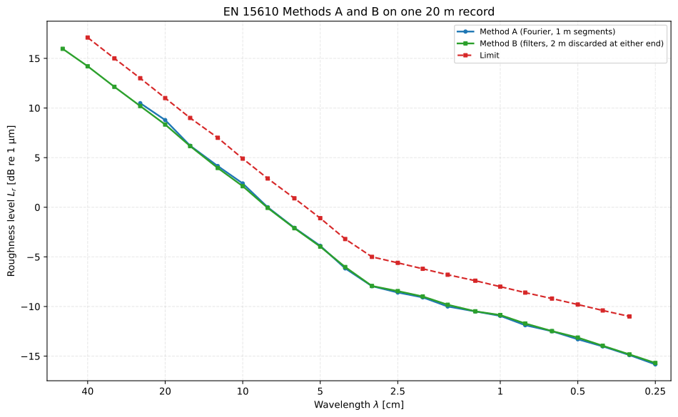
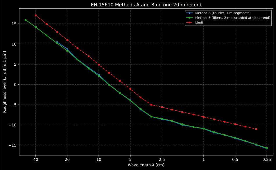
One record, two analyses: Method B reaches the 0,5 m band from 16 m of record, Method A stops at a quarter of its 1 m segments, and where both report they agree to the scatter of the estimate.
4.2 How fast vibration decays along the rail (EN 15461)
Section titled “4.2 How fast vibration decays along the rail (EN 15461)”The track decay rate is the attenuation of the vibration along the rail,
in decibels per metre, one value per one-third octave band (EN 15461, 3.6).
An accelerometer sits on the rail at the middle of a sleeper bay and a hammer
strikes the rail at the positions of Figure 2, every quarter bay out to two and
a half, then more sparsely, to 66 bays (6.7,
track_decay_excitation_positions). From the band magnitudes of
the responses, the direct one first, Formula 1 estimates the rate
from the integral of the squared response rather than from a fitted slope,
where is the length of rail each position stands for (Annex A). A grid that stops at cannot measure a rate below (Formula 2), and a band whose rate is not at least twice that is unsuitable; the farthest response also has to be 10 dB below the direct one (6.7).
bands = [100.0, 125.0, 160.0, 200.0, 250.0, 315.0, 400.0, 500.0, 630.0,         800.0, 1000.0, 1250.0, 1600.0, 2000.0, 2500.0, 3150.0, 4000.0, 5000.0]# The rates a ballasted track with concrete sleepers might have, dB/m.vertical = [9.0, 8.0, 6.0, 4.0, 3.0, 3.5, 7.0, 8.0, 7.0, 3.0, 1.2, 0.9, 0.9, 1.0, 1.1, 1.3, 1.5, 1.8]lateral = [6.0, 5.0, 4.0, 3.0, 3.0, 2.2, 1.2, 0.9, 0.7, 0.6, 0.5, 0.5, 0.6, 0.8, 0.9, 1.0, 1.2, 1.4]x_hammer = environment.track_decay_excitation_positions(sleeper_spacing_m=0.6)
def responses(rates_db_per_m):    """Exponentially decaying band magnitudes on the hammer grid, one row per position."""    beta = np.asarray(rates_db_per_m) / (20.0 * np.log10(np.e))    return np.exp(-np.outer(x_hammer, beta))
decay = [    environment.track_decay_rate(responses(vertical), frequencies_hz=bands, direction="vertical"),    environment.track_decay_rate(responses(lateral), frequencies_hz=bands, direction="lateral"),]print(x_hammer[-1], round(decay[0].minimum_measurable_db_per_m, 3), decay[1].far_field_sufficient)# 39.6 0.11 Trueprint(round(decay[0].rate_at(1000.0), 2), round(decay[1].rate_at(1000.0), 2))# 1.19 0.5
Formula 1 returns 1,19 dB/m for a response that decays at exactly 1,2 dB/m:
on the grid of Figure 2 the sum stands in for the integral, and it reads an
exponential about 1 % low. The limits are ISO 3095’s Figure 3, which prints
them in a table beside its curves, fourteen bands from 250 Hz to 5 kHz for each
direction (REFERENCE_TRACK_DECAY_LIMITS_DB_PER_M); below 250 Hz it sets
none.
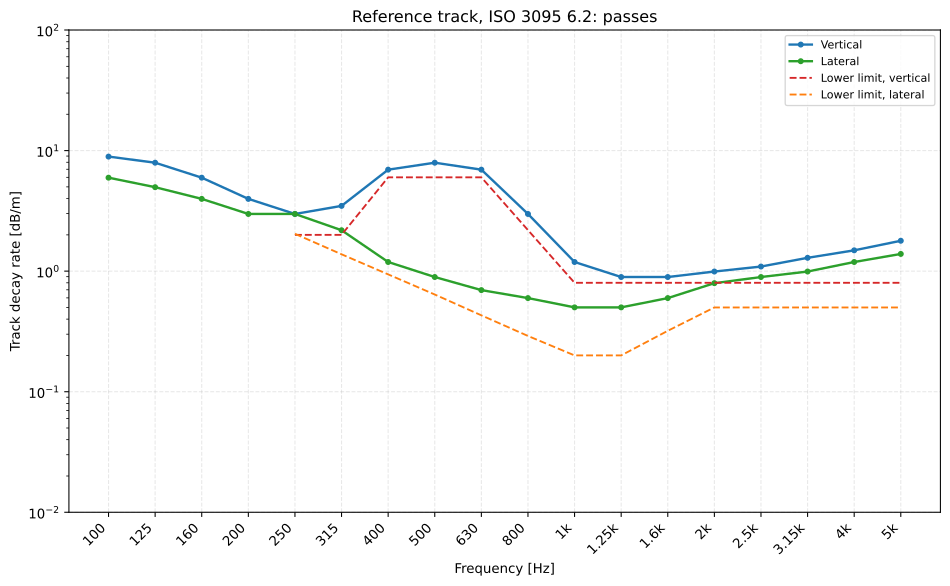
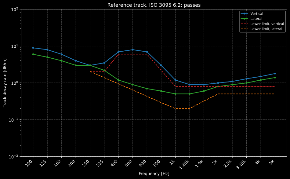
Both decay rates above the lower limits of Figure 3, the vertical one only just in the 1,25 kHz and 1,6 kHz bands.
4.3 The verdict
Section titled “4.3 The verdict”check_reference_track brings the two halves together with the geometry of
6.2.2 and returns one verdict, whose passes is the answer and whose
conditions are every requirement it judged, each with the clause it comes
from and the numbers it was judged on. When the decay rates come with their
grid, the floor of Formula 2 and the 10 dB drop of EN 15461 are judged too.
The verdict has no truth value of its own, so it cannot be tested with if
by mistake; the answer is .passes.
check = environment.check_reference_track( spectra, decay, speed_kmh=160.0, curve_radius_m=6000.0, track_gradient_ratio=0.002)print(check.passes)# Falsefor condition in check.failed: print(condition.clause, "|", condition.requirement, "|", condition.detail)# 6.2.5 | roughness at or below the limit of Figure 2 | exceeds by 2.4 dB at 0.0315 mEN 15610 clause 8 allows no band above the limit, and neither does 6.2.5 on its own. It adds one way out.
4.4 Small deviations: Annex C
Section titled “4.4 Small deviations: Annex C”Annex C accepts a track whose roughness exceeds the limit when the exceedance changes the pass-by level by no more than 1 dB, judged at each speed on a measured pass-by spectrum. The rails are averaged on their mean squares; the just-compliant spectrum is the measured one held down to the limit (Formula C.1); both are carried from wavelength to frequency at the train speed, , and their band energies redistributed over the normalised one-third octave bands, the synthesis of EN 15610 Annex C adapted to bands of unequal width; their difference is the correction (Formula C.2). The measured noise spectrum less that correction is the revised spectrum (Formula C.3), the least that could have been measured on a compliant track, and the effect is the energy sum of the measured spectrum less that of the revised one (Formula C.4):
noise = [68.0, 69.5, 71.0, 72.5, 74.0, 76.0, 78.0, 80.5, 83.0, 85.5, 87.0, 87.5, 86.5, 84.5, 82.0, 79.0, 75.5, 72.0] # L_pAeq,Tp(f) at 160 km/h, dBaverage = environment.average_roughness_spectra(spectra)small = environment.check_small_roughness_deviations( average, noise, frequencies_hz=bands, speed_kmh=160.0)print(round(small.impact_db, 2), small.passes)# 0.57 Truecheck = environment.check_reference_track( spectra, decay, speed_kmh=160.0, curve_radius_m=6000.0, track_gradient_ratio=0.002, small_deviations=small,)print(check.passes)# TrueAt 160 km/h the 5 cm to 2,5 cm bands land between 890 Hz and 1,8 kHz, which is
where this pass-by spectrum peaks, so the correction is 0,7 dB to 1,6 dB in
the three bands from 1 kHz to 1,6 kHz and the effect on the level is 0,57 dB:
the track is accepted for this vehicle at this speed. The same exceedance at
another speed falls on other frequencies and has to be judged again, and
check_reference_track refuses an Annex C verdict computed at another speed,
on anything but the quadratic average of the rails it judges (C.2.1), or
against any limit but the one it judges them against (Formula C.1).
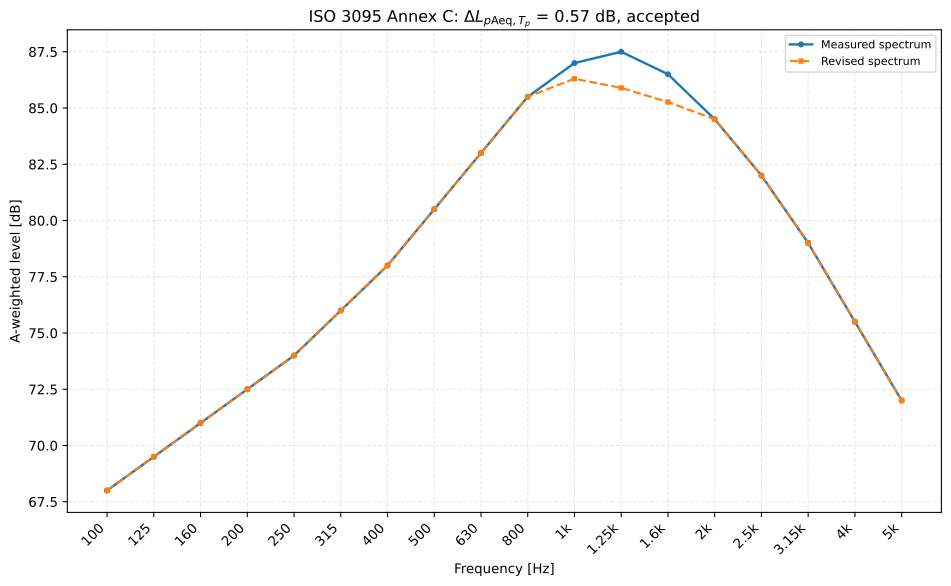
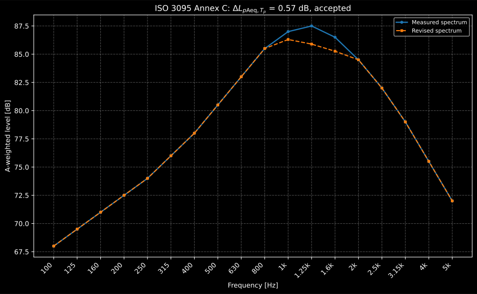
What the roughness above the limit could have added, band by band, and in total less than the 1 dB Annex C allows.
Show the code for these figures
import matplotlib.pyplot as plt
passby.plot()                     # the level history and the interval T_pcheck.plot(panel="roughness")     # the rails against Figure 2check.plot(panel="decay")         # the decay rates against Figure 3small.plot()                      # the Annex C spectraplt.show()
Annex E answers a neighbouring question, whether two test sites are
comparable in roughness: roughness_comparability forms the minimum and
maximum envelopes of their two roughness spectra (Formula E.1), carries each
through the Annex C chain against each site’s noise spectrum and bounds the
difference roughness alone could make in the pass-by level (Formulae E.4 and
E.5).
5. The uncertainty of Annex G
Section titled “5. The uncertainty of Annex G”Annex G treats the result as the reading plus uncorrelated corrections, so every sensitivity coefficient is 1 (Formulae G.1 and G.4); an input known only by its limits has (Formula G.2), the combined standard uncertainty is the root sum of squares (Formula G.5) and the expanded uncertainty is twice that (Formula G.6). Table G.2 works the budget of a standstill measurement through, and it is the numeric oracle of the module:
from phonometry import metrology
rows = [  # Table G.2: input, mean value correction and standard uncertainty, dB    ("cal, reference", 0.0, 0.14), ("cal, long term", 0.0, 0.04),    ("cal, supply voltage", 0.0, 0.06), ("cal, distortion factor", 0.105, 0.06),    ("slm, direction", 0.0, 0.25), ("slm, frequency", 0.0, 0.25),    ("slm, level linearity", 0.0, 0.46), ("calibrator, meteorological", 0.0, 0.14),    ("slm, wind screen", 0.06, 0.03), ("tripod", 0.0, 0.35),    ("distance", 0.0, 0.06), ("ground level", 0.515, 0.30), ("rounding", 0.0, 0.29),]budget = environment.pass_by_uncertainty(    55.0, [metrology.Quantity(v, u, name=n) for n, v, u in rows])print(round(budget.level_db, 2), round(budget.combined_uncertainty_db, 2),      round(budget.expanded_uncertainty_db, 2))# 55.68 0.83 1.66   Table G.2 prints 55,68, 0,83 and 1,66print(round(metrology.rectangular(0.0, 0.8).uncertainty, 2))# 0.46   the level linearity row of Table G.1, +/-0,8 dB over the square root of 3
Figure G.1 draws each input’s share of the variance, largest first, and the result draws the same bars in the same order; the conformance suite checks the order against the figure’s labels.
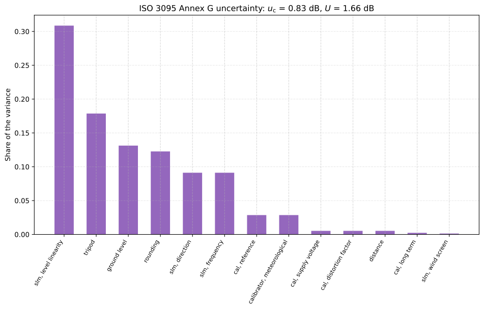
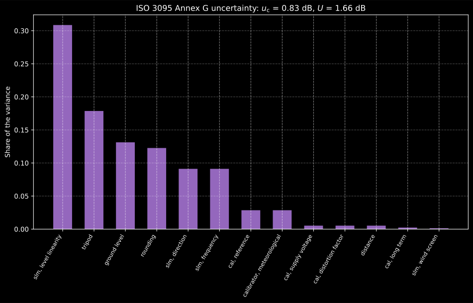
The budget of Table G.2 as Figure G.1 draws it: the linearity of the meter, the tripod and the ground carry three fifths of the variance.
Show the code for this figure
budget.plot()plt.show()6. The rest of the standard
Section titled “6. The rest of the standard”Three smaller pieces complete the tests. Annex A characterises impulsive noise by the steepest rise of over the stretches that climb without a break by at least 10 dB (Formula A.1). 6.3.4 accepts a vehicle coupled to the unit under test when it adds no more than 2,0 dB to the pass-by level, both levels rounded to one decimal. Annex D corrects a level for a steady background it stands more than 3 dB above (Formula D.1).
times = np.arange(0.0, 3.0, 0.01) # an L_pAF history every 10 mslevels = np.full(times.size, 70.0)levels[100:121] = 70.0 + 0.6 * np.arange(21) # 12 dB in 0.2 s, from 1 slevels[121:] = 82.0print(round(environment.impulsiveness_rise_speed(times, levels).rise_speed_db_per_s, 1))# 60.0 dB/sneutral = environment.check_adjacent_vehicle_neutrality(83.04, 81.06)print(neutral.difference_db, neutral.passes)# 1.9 Trueprint(round(environment.background_level_increase(78.0, 72.0), 2))# 1.26 dB the background adds to the 78 dB measured7. Where the printed text disagrees with itself
Section titled “7. Where the printed text disagrees with itself”The oracle rows of Table G.1 and Table G.2 do not all agree, and the
errata registry has the arithmetic of each:
the standard uncertainty of the 25 m microphone distance is printed as
0,004 dB where its interval gives 0,04 dB; the ground level at 7,5 m is
0,55 dB in Table G.1 and 0,30 dB in Table G.2, which Formula G.2 gives; and the
interval of the wind screen is printed with its bounds out of order. None of
them changes a number the library computes: the conformance rows read Table
G.2 as printed and hold the Table G.1 rows that Formula G.2 reproduces. In
EN 15610, the spike-removal loop of the Annex B listing repeats while any
second derivative is below the threshold, without the change of sign that
clause 7.2 c) also asks of a spike, so it never ends on a sharp bend of the
rail that is no spike at all. Neither it nor the clause’s “until no further
spike is detected”, read literally, ends on a peak that is detected and then
kept by the height test; the library ends the sweep when a pass removes
nothing, which is how it reads the clause. The same listing does Method B with
third-order Butterworth filters run forward and back (filtfilt), which
squares their response: 6,02 dB down just inside the band edges, where
Table 1 of EN 61260:1995 allows at most 5,5 dB for class 2, and a filter
integrated response of dB to dB, where 4.5.3 allows dB.
Clause 7.4.3 asks for filters that comply with EN 61260; the listing’s do not,
in any band or class, and read a band whose spectrum is flat about 0,6 dB low.
The library’s bank is class 0 on both.
What this guide covers
Section titled “What this guide covers”Covered
The computations of ISO 3095:2013 from measured records and levels:
pass_by_measurement(the equivalent level over any interval, the maximum with time weighting F, the record margins of 6.6.3 and the transit exposure level of ISO 3095:2005 or Formula B.1),transit_exposure_level,pass_by_time,stationary_unit_levelandstationary_test(Formulae 1 to 3 and 5.8.1),rolling_stock_testfor the constant-speed, starting and braking tests with the spread of 9.3,type_test_speeds,minimum_curve_radius,acceleration_test_positions,impulsiveness_rise_speed(Annex A),check_adjacent_vehicle_neutrality(6.3.4),background_level_increase(Annex D),check_small_roughness_deviations(Annex C),roughness_comparability(Annex E),check_reference_track(6.2) andpass_by_uncertainty(Annex G). From EN 15610:2009, the spike removal, the curvature processing, Method A with the band synthesis of Annex C, Method B with its filter bank graded against EN 61260:1995 (filtered_roughness_spectrum,roughness_filter_bank) and the 15 m it asks of each line, the average of 7.6 and the lines of 6.4.3; from EN 15461:2008+A1:2010, the decay rate of Formula 1 on the grid of Figure 2 with the floor of Formula 2 and the 10 dB drop. The limits of Figures 2 and 3 are read-only tables, and every result draws itself with.plot().Not covered
The measurement itself: laying out the stationary mesh, finding and inside a train, the site and weather checks, which are the tester’s, and the special cases of Annex B beyond Formula B.1. The speed normalisation 6.7.1 mentions, for which the standard gives no formula; the tonal difference, which 6.7.2 hands to ISO 1996-2 or DIN 45681; the platform, stopping-point and bridge measurements of Annex F. In EN 15610, the editing out of joints, welds and defects (Annex A shows what they look like; the operator does it), and the joining of records of 7.5. A record yields wavelengths up to a quarter of its length, which the library applies; to assess longer ones, 7.5 has the measured records concatenated by overlapping them, rules that “the overlap shall not be used for spectral components of 0,1 m or less” and asks for the concatenation method to be described in the report. It sets no length of overlap, no way to line two records up or to match their heights, no rule for how the samples they share are combined and no test that a join is valid (its NOTE only asks for attention to that), so the standard leaves the joining method to the tester, who must describe it in the report. In EN 15461, the measurement of the frequency response functions: the rates are computed from their band magnitudes. The roughness of the wheels, which the rail standards do not cover.
References
Section titled “References”- European Committee for Standardization. (2009). Railway applications — Noise emission — Rail roughness measurement related to rolling noise generation (EN 15610:2009). The rail roughness the reference track of ISO 3095 6.2.5 is judged by: the spike removal of 7.2, the curvature processing of 7.3, Method A of 7.4.2 with the band synthesis of Annex C, Method B of 7.4.3 with its filters held to EN 61260:1995, the average of 7.6 and the measurement lines of 6.4.3. Read from BS EN 15610:2009, which is identical to it.
- European Committee for Standardization. (2010). Railway applications — Noise emission — Characterisation of the dynamic properties of track sections for pass by noise measurements (EN 15461:2008+A1:2010). The track decay rates the reference track of ISO 3095 6.2.6 is judged by: the grid of Figure 2, the 10 dB drop of 6.7, Formula 1 and the floor of Formula 2, with Annex A. Read from BS EN 15461:2008+A1:2010, which is identical to it.
- International Organization for Standardization. (2005). Railway applications — Acoustics — Measurement of noise emitted by railbound vehicles (ISO 3095:2005). The second edition, read from BS EN ISO 3095:2005, which is identical to it: the transit exposure level of 3.14 and its Formulae 8 to 10, which the 2013 edition dropped.
- International Organization for Standardization. (2013). Acoustics — Railway applications — Measurement of noise emitted by railbound vehicles (ISO 3095:2013). The implemented edition (third edition, 2013-08-01): the stationary test of clause 5 and Formulae 1 to 3, the constant-speed test of clause 6 with the reference track of 6.2 and the limits Figures 2 and 3 print, the starting tests of clause 7 with the positions of Figure 10, the braking test of clause 8, the spread of 9.3, the rise speed of Annex A, Formula B.1, the small deviations of Annex C, the background correction of Annex D, the comparability of Annex E and the uncertainty budget of Annex G with its example, Table G.2.