Most of ISO 10140 measures what an element is: the sound reduction index of a wall, the impact level under a floor. Four of the application rules of ISO 10140-1 measure something else. Annex G measures what a lining adds to the wall it is fixed to, Annex H what a floor covering takes off the impact level of the floor it is laid on, Annex J what a joint lets through, a metre of it at a time, and Annex K what rain does to a roof, a roof window or a rooflight. The first two are products that are never sold on their own, so the laboratory measures the element twice, without and with the product, and reports the difference. A joint is a line rather than an area, measured in an element built to hide everything else. Rain is an impact source that falls from the sky rather than from a tapping machine, so the laboratory has to make its own rain.
The measurements themselves are the ones of Laboratory Insulation Measurement: to ISO 10140-2 and to ISO 10140-3, in a suite where flanking is suppressed. What this page adds is what the annexes do with them, and the single numbers that make two laboratories agree about a product whose effect depends on what it is fixed to.
Linings: the improvement ΔR (Annex G)
Section titled “Linings: the improvement ΔR (Annex G)”A lining is an additional layer on a wall or a ceiling: a plasterboard skin on studs, an external thermal insulation system, a dry lining glued to masonry. Annex G measures the basic element without and then with it and reports the sound reduction improvement index in every one-third-octave band,
(G.1). The improvement is not a property of the lining alone. It is only independent of the wall when the wall is much heavier than the lining, its critical frequency lies below the measured range and the two are weakly coupled (G.2); a lining on a lightweight wall behaves differently because the wall’s own coincidence moves the result. So G.2 names the walls to measure on: the standard basic elements of ISO 10140-5:2021 Annex B.
| Basic element | Construction | (; ) of its reference curve |
|---|---|---|
| Heavy wall | masonry or concrete of (350 ± 50) kg/m², critical frequency in the 125 Hz octave | 53 (−1; −5) dB |
| Heavy floor | the reinforced concrete slab of the heavyweight reference floor | 52 (−1; −5) dB |
| Lightweight wall | 10 cm aerated concrete of (600 ± 50) kg/m³ plastered, about 70 kg/m², critical frequency in the 500 Hz octave | 33 (−1; −2) dB |
The laboratory’s own wall is never exactly the reference one, so the single
number is not read off the two measured curves. ISO 717-1:2020 Annex D adds
the measured to the reference curve of the element,
(Formula (D.3)),
rates both curves, and takes the difference:
(Formula (D.4)). and
follow in the same way, and so does
every enlarged-range term of Annex B the measured bands reach. The result
carries the element as an index, or
. The reference curves are Table E.1 of
ISO 717-1:2020, published by the library as
building.LINING_REFERENCE_ELEMENTS; ISO 10140-5 printed the same numbers as
its Table B.1 until its 2021 edition moved them there.
import numpy as npfrom phonometry import building
freqs = [50, 63, 80, 100, 125, 160, 200, 250, 315, 400, 500, 630, 800,         1000, 1250, 1600, 2000, 2500, 3150, 4000, 5000]# The laboratory's heavy wall, and the same wall with plasterboard on# free-standing studs over mineral wool.r_without = np.array([36.1, 37.0, 38.2, 39.5, 40.3, 41.2, 40.6, 41.8, 43.9,                      46.4, 48.9, 51.6, 54.2, 56.5, 58.7, 61.4, 63.3, 64.2,                      64.8, 65.9, 66.4])delta_r = np.array([-2.1, -5.4, -3.2, 1.5, 4.8, 7.9, 10.6, 12.9, 14.7, 16.2,                    17.4, 18.3, 19.1, 19.6, 19.9, 19.5, 18.2, 16.4, 15.8,                    17.1, 18.0])res = building.lab_lining_improvement(r_without, r_without + delta_r, freqs,                                      basic_element="heavy_wall")rating = res.ratingprint(rating.index, rating.delta_rw, rating.delta_rw_c, rating.delta_rw_ctr)# heavy 12 11 10print(rating.without_lining.rating, rating.with_lining.rating)   # 53 65print(rating.delta_rw_c_50_3150, rating.delta_rw_ctr_50_3150)   # 9 3
The lining costs a few decibels at its mass-spring-mass resonance near 63 Hz and gains up to 20 dB above it; the traffic-weighted term, which leans on the low bands, gains least, and the enlarged-range sees the resonance itself and keeps only 3 dB.
On a wall that is not one of the three standard elements
(basic_element=None), Annex D has no reference curve to generalise with, and
G.2 c) allows only the direct difference of the measured single numbers,
(Formula (D.2)). It describes the lining on that wall in that laboratory and
nowhere else. The result carries it in every case, since it needs only the
two measured curves:
print(res.delta_rw_direct_db, res.delta_rw_c_direct_db, res.delta_rw_ctr_direct_db)# 13 12 9other = building.lab_lining_improvement(r_without, r_without + delta_r, freqs, basic_element=None)print(other.rating, other.delta_rw_direct_db) # None 13The octave values of G.1, where a report wants them, come from the three
thirds of each octave by ISO 717-1:2020 Formula (D.1),
, which
averages the transmission factors rather than the decibels, so the third that
improves least weighs most; res.octave_bands() returns them.
The wall must not change between the two measurements (G.4)
Section titled “The wall must not change between the two measurements (G.4)”is a difference of two measurements of the same wall, so the wall has to be the same wall both times. G.4 puts numbers on it for masonry and concrete: a curing period of at least two weeks before the first measurement, or, if the laboratory cannot wait, a time lag between the two measurements of at most one third of the curing time already elapsed. Its own example: two measurements carried out within one day can start three days after the end of construction.
check = building.check_lining_curing(10.0, 2.0) # daysprint(check.passes, check.cured, check.lag_within_third) # True False Trueprint(building.check_lining_curing(2.9, 1.0).passes) # FalseThe product specification may set another curing period
(required_curing_days=). The verdict has no truth value of its own: read
.passes, and .plot() draws the admissible region with the measurement in
it.
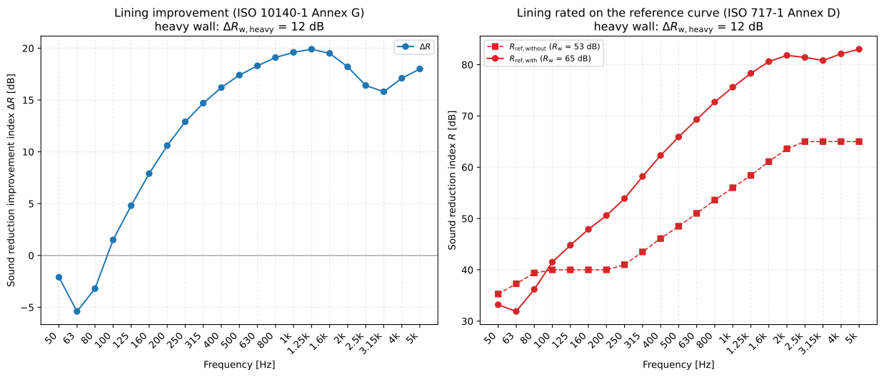
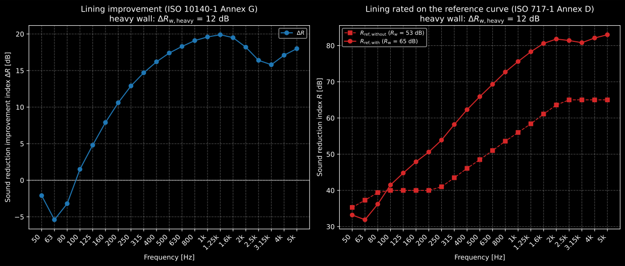
One plasterboard lining on the heavy wall. On the left the improvement the laboratory measured, band by band; on the right the two curves Annex D rates: the reference wall of Table E.1 and the same wall with the lining’s added. The 12 dB between their ratings is , a number that does not depend on the laboratory’s own wall.
Show the code for this figure
import matplotlib.pyplot as pltimport numpy as npfrom phonometry import building
freqs = [50, 63, 80, 100, 125, 160, 200, 250, 315, 400, 500, 630, 800,         1000, 1250, 1600, 2000, 2500, 3150, 4000, 5000]r_without = np.array([36.1, 37.0, 38.2, 39.5, 40.3, 41.2, 40.6, 41.8, 43.9,                      46.4, 48.9, 51.6, 54.2, 56.5, 58.7, 61.4, 63.3, 64.2,                      64.8, 65.9, 66.4])delta_r = np.array([-2.1, -5.4, -3.2, 1.5, 4.8, 7.9, 10.6, 12.9, 14.7, 16.2,                    17.4, 18.3, 19.1, 19.6, 19.9, 19.5, 18.2, 16.4, 15.8,                    17.1, 18.0])res = building.lab_lining_improvement(r_without, r_without + delta_r, freqs)
fig, (ax1, ax2) = plt.subplots(1, 2, figsize=(13, 5.6))res.plot(ax=ax1)res.rating.plot(ax=ax2)plt.tight_layout()plt.show()
Floor coverings: the improvement ΔL (Annex H)
Section titled “Floor coverings: the improvement ΔL (Annex H)”A floor covering (a carpet, a vinyl or rubber sheet, a floating screed, a parquet on an underlay) is laid on a reference floor and the tapping machine is run on it with and without the covering at the same positions. The improvement of impact sound insulation is
(Formula (H.1)) in each one-third-octave band, and the octave value comes from the three thirds by (Formula (H.2)), a mean of in which the third that improves least weighs most. As long as the receiving room’s absorption does not change between the two measurements, the reduction of is the reduction of (NOTE to H.1).
The reference floor matters more than it does for a lining, because a covering works against the stiffness of what is under it. ISO 10140-5:2021 Annex C builds one heavyweight floor, a reinforced concrete slab of 120 mm (+40/−20 mm, preferably 140 mm), and three lightweight (timber) floors that stand for the joist floors built around the world:
| Reference floor | Construction (ISO 10140-5:2021 C.2.1, C.3.3) | Reference curve | () |
|---|---|---|---|
| Heavyweight | concrete slab, 120 mm | 78 (−11) dB | |
| Lightweight No 1 | 22 mm chipboard on 120 mm × 180 mm joists at 625 mm, mineral wool, battens, 12,5 mm plasterboard | 72 (0) dB | |
| Lightweight No 2 | 20 mm OSB, plywood or chipboard on 42 mm × 225 mm joists at 610 mm, mineral wool, resilient channels, two layers of plasterboard | the same curve as No 1 | 72 (0) dB |
| Lightweight No 3 | two layers of 15 mm plywood on 45 mm × 60 mm joists at 300 mm over 120 mm × 240 mm beams at 1 m | 75 (−3) dB |
The curves are Table 4 of ISO 717-2:2020, published as
building.IMPACT_REFERENCE_FLOORS; the 2010 edition of ISO 10140-5 printed
them as its Table C.1. They are what the single number is read on, in the same
way as for a lining:
(ISO 717-2:2020 Formula (1)) and
(Formula (2)). On the heavyweight floor the result is
(Clause 5); on a lightweight floor it is ,
or (Clause 6), each with
its adaptation term or
(Formulas (A.4) and (A.6)).
freqs = [100, 125, 160, 200, 250, 315, 400, 500, 630, 800, 1000, 1250, 1600, 2000, 2500, 3150, 4000, 5000]# A resilient vinyl on the timber reference floor No 3.l_n0 = np.array([70.5, 73.4, 75.8, 77.2, 78.9, 78.1, 77.6, 78.3, 77.1, 75.4, 73.8, 71.2, 68.9, 65.7, 62.8, 59.6, 56.9, 53.8])delta_l = np.array([0.4, 0.8, 1.5, 2.3, 3.4, 4.9, 6.8, 9.1, 11.6, 14.2, 16.9, 19.8, 22.4, 25.1, 27.3, 29.4, 30.8, 31.9])cover = building.lab_floor_covering_improvement(l_n0, l_n0 - delta_l, freqs, reference_floor="lightweight_3")print(cover.designation, cover.delta_lw_db, cover.ci_delta_db) # ΔLt,3,w 8 -3print(cover.reference_rating.rating, cover.bare_rating.rating) # 67 75The two ratings at the end are the ones H.5 i) asks the report to state beside : the reference floor with the covering, , and the measured bare floor, . The same read on the heavyweight curve would give dB, because the concrete reference is loudest where the vinyl works best, at high frequency, and the timber one is loudest where it barely works at all. That is why ISO 717-2:2020 5.4 confines a measured on concrete to massive floors, and why a covering meant for timber floors is rated on a timber floor.
The two library functions that rate a spectrum directly,
weighted_impact_improvement and impact_improvement_adaptation_term, take the
same reference_floor= and, with one_decimal=True, the form ISO 717-2 5.4
prescribes when an uncertainty is stated beside the number.
Specimens, positions and loads
Section titled “Specimens, positions and loads”Annex H sorts coverings into three categories, and the category decides the specimen and the number of tapping-machine positions (H.2.2 and H.4.6):
- Category I, flexible coverings laid loose or glued (plastics, rubber, cork, matting): at least three small specimens of at least 650 mm × 350 mm, one tapping-machine position on each, hammers at least 100 mm from the edges. The bare floor may be measured at the same positions or with the machine either side of each specimen, averaging the two arithmetically; on a timber floor the line of hammers runs at 45° to the joists with at least one hammer over a joist.
- Category II, rigid or composite coverings, and category III, stretched coverings wall to wall: the whole floor or at least 10 m² with the shorter side at least 2,3 m; at least four machine positions on the heavyweight floor and six, randomly placed, on a lightweight one. A category II covering may be loaded with 20 kg/m² to 25 kg/m².
The floor surface should be between 18 °C and 25 °C (H.4.5). None of these conditions changes the arithmetic, and none is checked: they are what the test report has to state.
The rubber ball and the mock-up floor (H.6)
Section titled “The rubber ball and the mock-up floor (H.6)”H.6.1 measures the same covering under the heavy/soft impact source, the rubber ball of ISO 10140-5:2021 Annex F, and reports the reduction of its maximum level, (Formula (H.3)):
ball = building.heavy_impact_improvement([79.2, 73.5, 66.1, 58.4], [78.6, 71.9, 62.3, 51.0], [63, 125, 250, 500])print(ball.improvement_db) # [0.6 1.6 3.8 7.4]For a laboratory that cannot build a timber floor, H.6.2 allows a wooden
mock-up on the concrete slab instead (ISO 10140-5:2021 Annex G): a 22 mm
particleboard on twenty feet, loaded with five weights of 20 kg to 25 kg and
tapped at six fixed positions. Annex H names no reference curve for it, so its
describes the covering on a similar board, and the rating it is given
here is the one of the reference_floor the caller chooses.
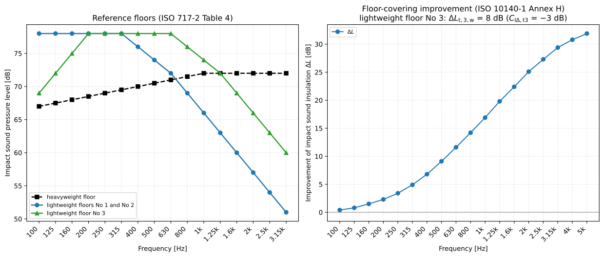
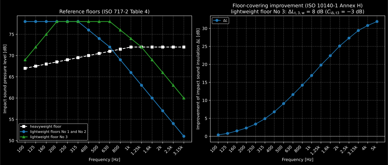
Left, the four reference floors, three curves because No 1 and No 2 share one. The concrete slab is loudest at high frequency; the joist floors are loudest below 400 Hz. Right, a resilient vinyl measured on floor No 3: an improvement that grows with frequency and is rated at only 8 dB on the timber curve, where the same spectrum would be rated at 18 dB on the concrete one.
Show the code for this figure
import matplotlib.pyplot as pltimport numpy as npfrom phonometry import building
freqs = [100, 125, 160, 200, 250, 315, 400, 500, 630, 800, 1000, 1250,         1600, 2000, 2500, 3150, 4000, 5000]l_n0 = np.array([70.5, 73.4, 75.8, 77.2, 78.9, 78.1, 77.6, 78.3, 77.1, 75.4,                 73.8, 71.2, 68.9, 65.7, 62.8, 59.6, 56.9, 53.8])delta_l = np.array([0.4, 0.8, 1.5, 2.3, 3.4, 4.9, 6.8, 9.1, 11.6, 14.2, 16.9,                    19.8, 22.4, 25.1, 27.3, 29.4, 30.8, 31.9])cover = building.lab_floor_covering_improvement(l_n0, l_n0 - delta_l, freqs,                                                reference_floor="lightweight_3")
fig, (ax1, ax2) = plt.subplots(1, 2, figsize=(13, 5.6))floors = building.IMPACT_REFERENCE_FLOORSx = np.arange(16)for key, style in (("heavyweight", "s--"), ("lightweight_1", "o-"),                   ("lightweight_3", "^-")):    ax1.plot(x, list(floors[key].values()), style, label=key)ax1.set_xticks(x, [f"{f:g}" for f in floors["heavyweight"]], rotation=45)ax1.set(xlabel="Frequency [Hz]", ylabel="Impact sound pressure level [dB]",        title="Reference floors (ISO 717-2 Table 4)")ax1.legend()cover.plot(ax=ax2)plt.tight_layout()plt.show()
The form of Figure H.4
Section titled “The form of Figure H.4”H.6.3 prints “an example of the form for the expression of results” and lets
the user copy it. cover.report() fills it: the manufacturer and product, the
client, the test room, who mounted the specimen, the date, the description of
facility and specimen, the type of reference floor, the mass per unit area,
the curing time, the air temperature and humidity in the source room and the
receiving room volume; the one-third-octave table of and
beside the diagram with the frequency range of the
ISO 717-2 rating dashed, as key 1 of the form marks it; and the rating, with
the two floor ratings H.5 i) asks for beside it. The product identification
and the curing time come from the product and curing_time_h fields of
ReportMetadata.
from phonometry import ReportMetadata
cover.report("covering.pdf", metadata=ReportMetadata(    manufacturer="Example floorings", product="Resilient vinyl, 4 mm",    mass_per_area=2.6, curing_time_h=0.0, source_temperature_c=21.2,    source_relative_humidity_percent=48.0, receiving_volume=58.0))
The form also asks for , a term of the reference floor with the covering from 50 Hz, which the reference floors of ISO 717-2:2020 Table 4 cannot give: they start at 100 Hz (see the errata registry). The sheet says so where the number would go.
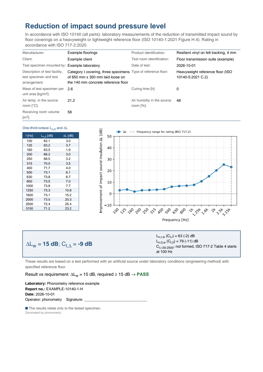
The form of ISO 10140-1:2021 Figure H.4 filled with the floor and the covering of ISO 717-2:2020 Annex C: the header with manufacturer, product, type of reference floor, mass per unit area, curing time and the climate of the source room, the one-third-octave table of Ln,0 and delta L beside the delta L diagram with the frequency range of the ISO 717-2 rating dashed, the boxed delta Lw = 15 dB with CI,delta, the two floor ratings of H.5 i), the note on CI,r,50-2500 and a PASS verdict.
Joints: the sound reduction index per metre (Annex J)
Section titled “Joints: the sound reduction index per metre (Annex J)”A joint is a line, not an area: a slit with or without a filler, a foam or sealing tape between two elements, the gasket on the rebate of a door or a window. Annex J measures what it lets through. The joint is mounted in an element that insulates far better than it does, the level difference is measured to ISO 10140-2, and the result is normalized to a metre of joint rather than to a square metre of element,
(Formula (J.1)), with the joint length , the equivalent absorption area of the receiving room, m² and m. A joint twice as long lets twice the power through and lowers the level difference by 3 dB; the term in gives the 3 dB back, which leaves a number that does not depend on how much of the joint the laboratory could fit in its opening.
# One band: 95 dB in the source room, 48.6 dB in the receiving room, whose# absorption area is 12.4 m2, with 5.4 m of rebate seal in the opening.r = building.joint_sound_reduction_index([95.0], [48.6], [12.4], joint_length_m=5.4)print(np.round(r, 1)) # [42.8]The element around the joint is part of every measurement (J.1)
Section titled “The element around the joint is part of every measurement (J.1)”Whatever the joint lets through, the element it sits in lets something through too, and a good seal can come close to it. So J.1 asks for the maximum of the arrangement, : the same Formula (J.1) with the joint sealed on both sides, “e.g. with elastic sealant”. Unless the maximum lies at least 10 dB above the measured index , the result is corrected by the rules of ISO 10140-2:2021 A.3, band by band, with :
| Margin | |
|---|---|
| 10 dB or more | , no correction |
| 6 dB to 10 dB | , Formula (J.2) |
| under 6 dB | dB, a minimum value |
| under 3 dB | , in brackets |
The 1,3 dB is what Formula (J.2) gives at 6 dB, which is how A.3 puts it. A.3
itself stops correcting a sound reduction index at 15 dB and an
element-normalized level difference at 10 dB; Annex J writes the 10 dB, which
fits an index normalized to a reference length rather than to the area of
the opening, and the 10 dB is what the library applies. The
last row is exact rather than cautious: the arrangement passes the power of
the maximum alone, and the power of the joint on top of it when the joint is
open, so a measured index within 3 dB of the maximum means the joint passes
less than the element does, and its own index is above .
J.1 allows that lower limit (“may be set”); limit_at_maximum=False gives
those bands the 1,3 dB instead.
A rebate seal on a door, measured against its arrangement:
freqs = [100, 125, 160, 200, 250, 315, 400, 500, 630, 800, 1000, 1250, 1600, 2000, 2500, 3150, 4000, 5000]r_max = np.array([40.2, 42.8, 45.1, 48.6, 51.9, 54.3, 56.8, 58.9, 60.7, 62.4, 63.8, 65.1, 66.2, 67.0, 67.6, 68.1, 68.5, 69.0])r_seal = np.array([33.4, 35.1, 37.9, 40.6, 43.0, 45.2, 46.1, 46.8, 47.0, 46.2, 45.1, 46.9, 49.8, 52.6, 55.4, 58.9, 63.1, 66.2])seal = building.lab_joint_insulation(r_seal, r_max, freqs, joint_length_m=5.4)print(seal.regime[-4:])# ('uncorrected', 'corrected', 'limit', 'maximum')print(np.round(seal.r_s_db[-4:], 1)) # [55.4 59.5 64.4 69. ]The single numbers are those of ISO 717-1 on the corrected index, and the form of Figure J.7 asks for the enlarged-range terms to 5 000 Hz as well:
rating = seal.ratingprint(rating.rating, rating.c, rating.ctr) # 49 -1 -4print(seal.c_100_5000_db, seal.ctr_100_5000_db) # 0 -4print(seal.max_rating.rating) # 61Where a band is above dB, it says only that the joint is better than the arrangement can show. J.1 rates the curve a second time with an infinitely high index in those indicative bands, which then add no unfavourable deviation and no energy, and if the two ratings differ by more than 1 dB the single numbers go in brackets too. Here the only indicative band is 5 000 Hz, outside the rating range, so nothing moves:
print(seal.open_band_rating.open_frequencies_hz, seal.bracketed) # (5000.0,) Falseseal.octave_bands() averages the transmitted power of the three thirds of
each octave, the octave index Figure J.9 plots.
The test element and the gap width (J.2)
Section titled “The test element and the gap width (J.2)”J.2.1 asks for a joint longer than 1 m and no wider than 50 mm, and J.2.2 for at least 5,0 m of a gap between the parts of a window or door, which may be the sum of several gaps. The gap width is read at four positions or more, evenly spread along the seal, and the readings “shall not deviate by more than 0,3 mm, otherwise readjust the mounting”; their average is the gap width.
check = building.check_joint_test_element(5.4, 5.0, window_or_door_gap=True)print(check.passes) # Truegap = building.check_gap_width([5.1, 4.9, 5.0, 5.15, 4.95])print(round(gap.gap_width_mm, 2), round(gap.spread_mm, 2), gap.passes)# 5.02 0.25 TrueThe deviation is read between the readings, the largest minus the smallest:
the sentence could also mean each reading against the average, which would let
the readings spread twice as far, and the stricter reading is the one checked.
Both verdicts have no truth value of their own: read .passes.
A variable slit (J.4 and J.5)
Section titled “A variable slit (J.4 and J.5)”An openable window or door does not have one gap width, so J.4 repeats the test at three: the nominal width the manufacturer gives (5 mm when it gives none), the minimum width under the maximal pressure (normally a force of 100 N per metre of seal), and mm. The report then gives every single number as a function of the gap width with the nominal width marked (J.5.2 i)), and the results at and are the ones products are compared by (J.5.2 h)).
loss = {3.0: -2.5, 4.0: -1.2, 5.0: 0.0, 6.0: 2.5, 8.0: 8.0, 10.0: 12.5, 12.0: 13.0} # dB lost against 5 mm, mid bandslope = np.linspace(0.6, 1.4, 18) # and more at high frequencyresults = [building.lab_joint_insulation( np.minimum(r_seal - db * slope, r_max - 0.5), r_max, freqs) for db in loss.values()]series = building.joint_gap_series(list(loss), results, minimum_gap_mm=3.0)print(series.r_s_w_ctr_db) # [48. 47. 45. 43. 38. 33. 33.]print(series.at_gap(7.0), series.working_range_mm) # 40.5 (5.0, 8.0)at_gap reads the straight line between the two measured widths either side,
as Figure J.8 draws “lines plotted through measurement results”, and never
extrapolates. Where J.5.2 h) lets “a gap range other than 3 mm” apply, it reads
the single numbers at that width as well; working_range_mm and the figure
keep the 3 mm that J.4 c) measures at. series.plot_octave_bands() draws
Figure J.9: the octave index at every gap width, under the closed and sealed
element () as , which J.5.1 says the figure also
gives.
joint_gap_series collects any set of widths; whether the three of J.4 are
among them is a verdict of its own. J.4 gives no tolerance, so a width within
the 0,3 mm that J.2.2 lets the readings of a gap width spread over counts as the
width asked for, and a series that does not name fails J.4 b),
since nothing then shows which width it was.
widths = building.check_joint_gap_series(series)print(widths.nominal_measured, widths.minimum_measured, widths.working_range_measured, widths.passes) # True True True True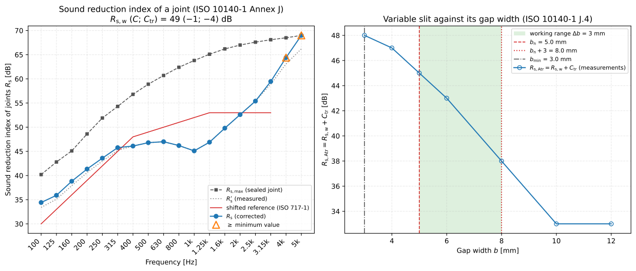
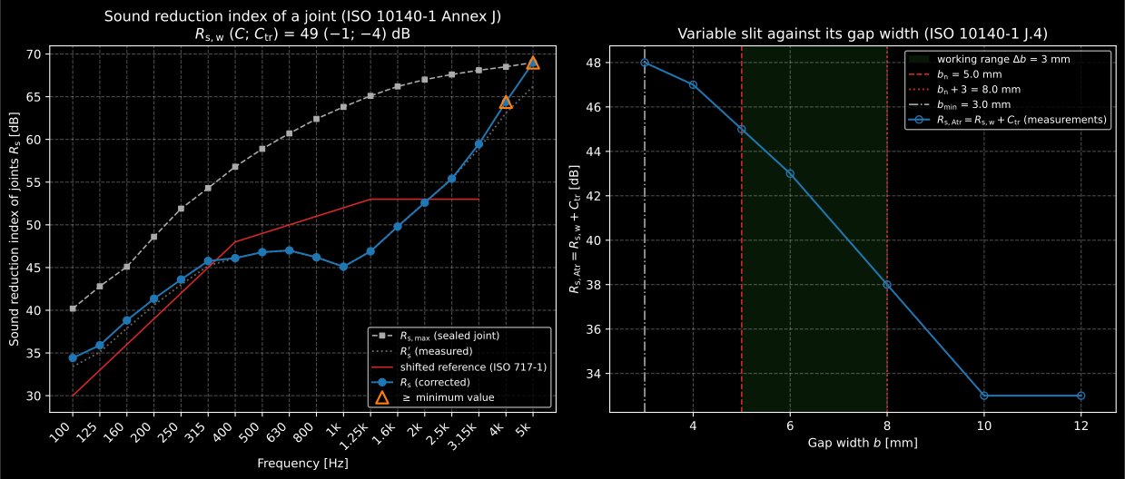
Left, the seal at its nominal gap: the measured index, the maximum of the arrangement above it, and the corrected index, whose two top bands are minimum values because the seal comes within 6 dB and then within 3 dB of what the arrangement can show. Right, the same seal at seven gap widths: 7 dB of are lost across the 3 mm working range from the nominal width.
Show the code for this figure
import matplotlib.pyplot as pltimport numpy as npfrom phonometry import building
freqs = [100, 125, 160, 200, 250, 315, 400, 500, 630, 800, 1000, 1250,         1600, 2000, 2500, 3150, 4000, 5000]r_max = np.array([40.2, 42.8, 45.1, 48.6, 51.9, 54.3, 56.8, 58.9, 60.7, 62.4,                  63.8, 65.1, 66.2, 67.0, 67.6, 68.1, 68.5, 69.0])r_seal = np.array([33.4, 35.1, 37.9, 40.6, 43.0, 45.2, 46.1, 46.8, 47.0, 46.2,                   45.1, 46.9, 49.8, 52.6, 55.4, 58.9, 63.1, 66.2])seal = building.lab_joint_insulation(r_seal, r_max, freqs, joint_length_m=5.4)loss = {3.0: -2.5, 4.0: -1.2, 5.0: 0.0, 6.0: 2.5, 8.0: 8.0, 10.0: 12.5,        12.0: 13.0}slope = np.linspace(0.6, 1.4, 18)results = [building.lab_joint_insulation(               np.minimum(r_seal - db * slope, r_max - 0.5), r_max, freqs)           for db in loss.values()]series = building.joint_gap_series(list(loss), results, minimum_gap_mm=3.0)
fig, (ax1, ax2) = plt.subplots(1, 2, figsize=(13, 5.6))seal.plot(ax=ax1)series.plot(ax=ax2)plt.tight_layout()plt.show()
The form of Figure J.7
Section titled “The form of Figure J.7”J.5.1 prints a sample form for the result and J.5.2 b) asks the report for “a
data sheet with a diagram which shows the sound insulation of joints as a
function of the frequency”. seal.report() writes it: the header of the form
(client, specimen, date, test length, separation wall, test noise, room
volumes, the maximum joint sound reduction index, mounting, and the climate of
both rooms), the table of from 100 Hz to 5 000 Hz beside its
diagram over the printed 30 dB to 80 dB, with ≥ before a minimum value and
brackets round one set to the maximum, and the evaluation
(; ), and
. When J.1 puts the single numbers in brackets,
every one of them is, and a note gives each of them rated with the indicative
bands open, so the one that moved is there to see. The separation wall and the
test noise come from the separating_element and test_signal fields of
ReportMetadata; the climate comes from the per-room fields when they are
given.
seal.report("joint.pdf", metadata=ReportMetadata( client="Example client", separating_element="Lead-lined filler wall", test_signal="Pink noise", source_volume=53.0, receiving_volume=51.0))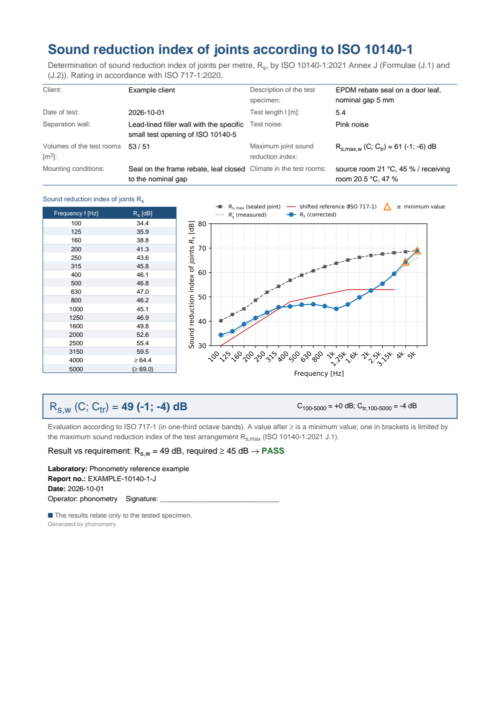
The form of ISO 10140-1:2021 Figure J.7 for an EPDM rebate seal: the header with the test length, the separation wall, the test noise, the room volumes and the maximum joint sound reduction index of the arrangement, the one-third-octave table of Rs from 100 Hz to 5000 Hz beside its diagram, with the 4000 Hz band as a minimum value and the 5000 Hz band in brackets at the maximum, the boxed Rs,w (C; Ctr) with C100-5000 and Ctr,100-5000, and a PASS verdict.
Rain on a roof (Annex K)
Section titled “Rain on a roof (Annex K)”Rain is impact sound. It is measured as the sound intensity level that the roof, roof window or rooflight radiates into the room below: sound power per unit area, re W/m² (K.1). Per unit area, because on a large roof only part of the surface is wet, and the power grows with the area the rain actually strikes.
The rain
Section titled “The rain”Natural rain is classed by rate, drop size and fall velocity (Table K.1, after
IEC 60721-2-2:1988): moderate up to 4 mm/h, intense up to 15 mm/h, heavy up to
40 mm/h and cloudburst above 100 mm/h, published as
building.RAINFALL_CLASSIFICATION. The laboratory reproduces two of them at
their upper limits, “since larger drops produce most of the sound generated”
(ISO 10140-5:2021 H.1), with a tank whose perforated base drops water from a
fixed height (Tables H.1 and H.2, building.ARTIFICIAL_RAIN):
| Artificial rain | Rainfall rate | Volume median drop diameter | Fall velocity | Holes and fall height |
|---|---|---|---|---|
| Intense (optional) | 15 mm/h | 2,0 mm | 4,0 m/s | 0,3 mm to 0,5 mm, about 25 per m², about 1 m |
| Heavy (mandatory) | 40 mm/h | 5,0 mm | 7,0 m/s | 1 mm, about 60 per m², about 3,5 m |
Heavy rain is the one products are compared under (K.4.1). The generator is checked by its rate, which “shall be within ±2 mm/h” of the table; for a generator that is not the tank of Table H.2, half of the drops should also lie within ±0,5 mm of the median diameter and within ±1 m/s of the fall velocity. The rate is measured by collecting the water, one litre per square metre being one millimetre:
rate = building.rainfall_rate(3.1, 0.08, 3600.0) # litres, m², sprint(rate) # 38.75 mm/hcheck = building.verify_rain_generator(rate, rain_type="heavy")print(check.passes, check.rate_deviation_mm_h) # True -1.25The level
Section titled “The level”With the rain falling steadily for at least 5 min, the room-averaged sound pressure level and the reverberation time of the test room are measured to ISO 10140-4 and turned into the intensity level
(Formula (K.1), s, m³, m²). The constant is the
diffuse-field sound power of a room with the Sabine area ,
dB, and is the area the rain
excites: the whole specimen for a roof window or rooflight of about
1,25 m × 1,5 m, and three times the perforated area of the tank for a large
roof of 10 m² to 20 m², which is rained on from three positions whose levels
are added energetically (K.4.2). The 18 bands from 100 Hz to 5000 Hz combine
into the A-weighted level,
(Formula (K.2)), whose 18 corrections of Table K.2 are the A-weighting
of IEC 61672-1:2013, the frequency weighting
of the library, at the exact midband frequencies of the bands, rounded to
0,1 dB (building.RAINFALL_A_WEIGHTING).
K.4.3 allows the intensity to be measured directly with a probe over a surface
instead,
(Formula (K.4), rainfall_sound_from_intensity).
Normalized to the reference pane
Section titled “Normalized to the reference pane”Two laboratories with the same tank still disagree, because their rain and their mountings differ. K.6 therefore measures a reference specimen first: a single 6 mm glass pane of 1,25 m × 1,5 m, mounted as a window pane and centred under heavy rain (ISO 10140-5:2021 Annex I). Its structural reverberation time gives its loss factor, (Formula (I.1)); its level is brought to the reference loss factor of Table I.1, (Formula (I.2)), and the difference from the reference level of the same table is the laboratory’s correction, (Formula (I.3)). Every specimen is then reported normalized, (Formula (K.5)).
freqs = [100, 125, 160, 200, 250, 315, 400, 500, 630, 800, 1000, 1250,         1600, 2000, 2500, 3150, 4000, 5000]# The reference pane, mounted a little more lossily than Table I.1 assumes.l_i_ref = np.array([46.2, 45.8, 46.9, 46.5, 47.8, 47.2, 47.9, 48.1, 47.6,                    46.8, 44.9, 43.1, 43.8, 46.9, 51.6, 50.9, 46.8, 44.6])t_s = np.array([0.176, 0.177, 0.138, 0.139, 0.140, 0.111, 0.111, 0.088,                0.088, 0.070, 0.070, 0.071, 0.055, 0.056, 0.044, 0.044,                0.035, 0.035])correction = building.rainfall_reference_correction(l_i_ref, t_s)
# A polycarbonate rooflight of 1.25 m x 1.5 m under heavy rain, 62 m3 room.l_pr = np.array([48.2, 51.0, 53.1, 55.4, 57.0, 58.3, 59.1, 59.8, 60.2, 60.4,                 60.1, 59.4, 58.6, 57.5, 56.2, 54.4, 52.3, 49.8])t = np.array([1.9, 1.8, 1.7, 1.6, 1.5, 1.45, 1.4, 1.35, 1.3, 1.25, 1.2, 1.15,              1.1, 1.05, 1.0, 0.95, 0.9, 0.85])rain = building.rainfall_sound(l_pr, t, freqs, volume_m3=62.0,                               excited_area_m2=1.875,                               reference_correction=correction)print(round(rain.l_ia_db, 1), round(rain.l_ia_norm_db, 1))     # 69.3 67.5print(rain.octave_bands()[0])       # [ 125.  250.  500. 1000. 2000. 4000.]
K.5 e) asks for , , and
to 0,1 dB with the rainfall rate beside them. The sound
power the whole specimen radiates follows from the NOTE to Formula (K.2),
, as rain.sound_power_levels(area_m2).
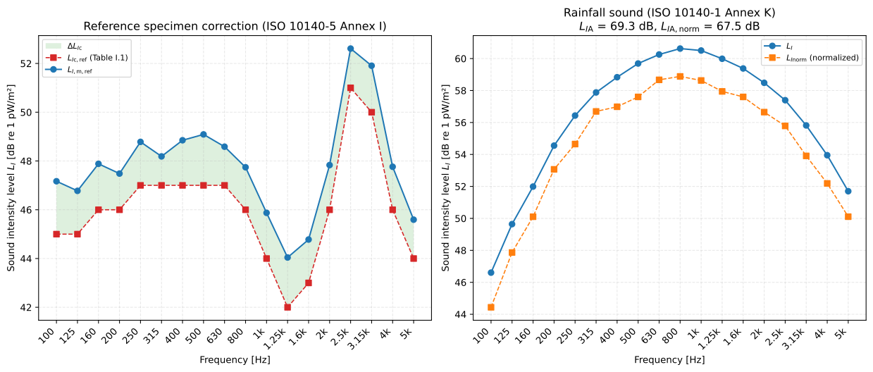
Left, the laboratory’s reference pane, corrected to the reference loss factor, against the reference level of Table I.1: the shaded gap is the correction every later specimen is normalized by. Both curves peak at 2500 Hz, just above the coincidence frequency of a 6 mm pane. Right, a rooflight under heavy rain: the intensity level as measured and normalized, and its A-weighted totals.
Show the code for this figure
import matplotlib.pyplot as pltimport numpy as npfrom phonometry import building
freqs = [100, 125, 160, 200, 250, 315, 400, 500, 630, 800, 1000, 1250,         1600, 2000, 2500, 3150, 4000, 5000]l_i_ref = np.array([46.2, 45.8, 46.9, 46.5, 47.8, 47.2, 47.9, 48.1, 47.6,                    46.8, 44.9, 43.1, 43.8, 46.9, 51.6, 50.9, 46.8, 44.6])t_s = np.array([0.176, 0.177, 0.138, 0.139, 0.140, 0.111, 0.111, 0.088,                0.088, 0.070, 0.070, 0.071, 0.055, 0.056, 0.044, 0.044,                0.035, 0.035])correction = building.rainfall_reference_correction(l_i_ref, t_s)l_pr = np.array([48.2, 51.0, 53.1, 55.4, 57.0, 58.3, 59.1, 59.8, 60.2, 60.4,                 60.1, 59.4, 58.6, 57.5, 56.2, 54.4, 52.3, 49.8])t = np.array([1.9, 1.8, 1.7, 1.6, 1.5, 1.45, 1.4, 1.35, 1.3, 1.25, 1.2, 1.15,              1.1, 1.05, 1.0, 0.95, 0.9, 0.85])rain = building.rainfall_sound(l_pr, t, freqs, volume_m3=62.0,                               excited_area_m2=1.875,                               reference_correction=correction)
fig, (ax1, ax2) = plt.subplots(1, 2, figsize=(13, 5.6))correction.plot(ax=ax1)rain.plot(ax=ax2)plt.tight_layout()plt.show()
How the measurement goes
Section titled “How the measurement goes”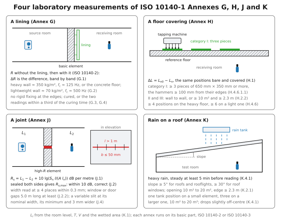
A lining. Build the basic element in the test opening (the heavy wall, the heavy floor or the lightweight wall of ISO 10140-5 Annex B, or the wall of interest), let it cure, and measure to ISO 10140-2. Fix the lining as it would be fixed in practice, with no stiff connection to the laboratory’s flanking elements (G.3), let it reach its final condition, and measure within the G.4 time lag. Report both curves, the improvement, the single numbers with the element index, and the element’s mass and construction (G.5).
A floor covering. Measure on the bare reference floor to ISO 10140-3, lay the covering by category, and measure at the same tapping-machine positions. Report the category, the specimen, the positions, the load, the floor temperature, with its weighted value and adaptation term, and the two ratings of H.5 i).
A joint. Build the joint into an element that insulates far better than it does, at least 1 m long and no wider than 50 mm (5,0 m for a gap between the parts of a window or door), read the gap width at four positions or more, and measure , and the reverberation time to ISO 10140-2. Seal the joint on both sides and measure the arrangement’s maximum the same way. A variable slit is measured again at its minimum width under load and at its nominal width plus 3 mm. Report the maximum, the data sheet of Figure J.7 for each gap width, the test element and the cross-section with its gap width, and the single numbers against the gap width (J.5.2).
Rain. Install the specimen at its slope (at least 5° for roofs and rooflights, 30° for roof windows) in an opening of 10 m² to 20 m², or a roof window in a heavy filler construction; check the rain rate; rain on it steadily for 5 min before measuring; measure , and the background, from one generator position or three; and normalize with the laboratory’s own reference pane. Report the rain type and rate, the generator and its position, and to 0,1 dB, and the A-weighted totals (K.5).
Verifying it
Section titled “Verifying it”The printed tables and examples of the four annexes, and the tables behind them, are conformance rows:
-
The reference curves, band by band: the 63 values of ISO 717-1:2020 Table E.1 and the 48 of ISO 717-2:2020 Table 4, against a reading of the page kept apart from the library, and the single numbers under them: the nine terms of Table E.1 under each of the three basic elements, integer and to one decimal place (54 numbers), and with under each of the three curves of Table 4, both forms (12 numbers), which the published curves reproduce through the ISO 717 rating engine. The band values are needed as well as the single numbers, because a single number does not move with every band: a decibel mistyped at 4 000 Hz of the heavy floor changes none of them.
-
A sloped improvement on every reference floor and a sloped lining on every standard element, rated by a separate implementation of the printed clauses of ISO 717-1 and ISO 717-2: a flat spectrum gives the same number on every curve, and the same as , while a sloped one tells them apart. The direct differences of Formula (D.2) are checked on the same sloped lining. A second lining, with its mass-spring-mass resonance at 100 Hz and a coincidence dip at 4 000 Hz, puts weight on the bands 50 Hz to 80 Hz and 4 000 Hz to 5 000 Hz that set the enlarged ranges apart: rated the same way, it gives every two of the nine lining terms different numbers on at least one element, so no two of them could be swapped unseen.
-
The 18 of Table K.2 against the A-weighting of IEC 61672-1 at the exact midband frequencies, rounded to 0,1 dB: all 18 agree. The same 18 values, as printed, also carry a flat spectrum through Formula (K.2), so a mistyped in the published table would show in .
-
The ISO 717-2 Annex C example, carried end to end through the Annex H front end: dB as printed, and dB from the Table 4 floor, where the example’s own chain gives −8 dB (see the errata registry).
-
The G.4 example: measurements within 1 d that start 3 d after construction pass, and 2,9 d fails. The bound is inclusive on any input: 2,1 d after 6,3 d passes as well, although 3 × 2,1 comes out a rounding error above 6,3 in binary arithmetic.
-
Tables K.1, H.1, H.2 and I.1 cell by cell as printed, and Formulas (I.1) to (I.3) on a pane at twice the reference loss factor of the printed Table I.1, which has to come out dB in all 18 bands.
-
The H.1 tolerance at its bounds, which it includes: 38 mm/h passes, also when it comes out of
rainfall_rateas 3,8 L collected on 0,1 m² in one hour, a rounding error below 38. Then Formula (K.1) with every term away from zero, and closed forms of Formulas (D.4) and (K.4). -
Annex J at its printed numbers: the fixed 1,3 dB below a 6 dB margin is Formula (J.2) at 6 dB to the printed decimal, as ISO 10140-2:2021 A.3 says it corresponds, and the library applies exactly that just below it; the lower limit J.1 prints as its example, dB in brackets; and the typical flanking spectrum of ISO 10140-2:2021 Table A.1 carried through the joint front end, rated 59 (; ) dB as printed. Then Formula (J.1) with every term away from zero, the bounds of J.2.1 and J.2.2 at their printed values, each inclusive or exclusive as the text says, the three gap widths of J.4 with the 5 mm taken when the nominal width is unknown and the 3 mm above it, and the open-band rating checked by hand against ISO 717-1 Clauses 4.4 and 4.5.
The rain has no worked example in either standard, so Formulas (K.1) to (K.5) are checked in closed form rather than against a printed result. Tables H.1 and I.1 were read on the pages of the 2021 edition and agree digit for digit with the 2010 edition and its 2014 amendment, where they first appeared.
Quick answers
Section titled “Quick answers”Is ΔRw the difference of the two measured Rw?
Section titled “Is ΔRw the difference of the two measured Rw?”Only on a wall that is not a standard basic element, where it is . On a standard element the measured is added to the element’s reference curve and the two reference ratings are subtracted, which removes the particular wall of the laboratory from the number. In the example above the two differ by a decibel, 12 dB against 13 dB.
Why is my covering 18 dB on concrete and 8 dB on timber?
Section titled “Why is my covering 18 dB on concrete and 8 dB on timber?”Because the two ratings read the same against different reference floors. The concrete reference curve is loudest at high frequency, where a resilient covering works best; the timber curves are loudest below 400 Hz, where it barely works. A measured on concrete applies to massive floors only (ISO 717-2:2020 5.4).
Why is a band of my joint in brackets?
Section titled “Why is a band of my joint in brackets?”Because the joint came within 3 dB of what the arrangement can show there, so the measurement says only that the joint is better than : the band is reported as . A better filler wall or a better seal on the sealed measurement raises the maximum and turns the band into a number. If such bands also move the single numbers by more than 1 dB, the single numbers go in brackets too (J.1).
Do I need the reference pane to report rain noise?
Section titled “Do I need the reference pane to report rain noise?”The intensity level and are reported without it. The normalized levels, which are what makes two laboratories comparable, need the laboratory’s own reference measurement (K.6, K.5 f)). No reference specimen is defined for large roofs (ISO 10140-5:2021 I.3).
Standards
Section titled “Standards”Covered
ISO 10140-1:2021 Annex G: the sound reduction improvement index of G.1, its octave values, the single numbers , and with every enlarged-range term on the three standard basic elements (ISO 717-1:2020 Annex D, Formulae (D.1) to (D.4)), the direct differences of Formula (D.2), and the curing condition of G.4. Annex H: of Formula (H.1), the octave values of Formula (H.2), the weighted reductions and with and on all four reference floors (ISO 717-2:2020 Clauses 5 and 6, A.2.2, A.2.3), the two ratings of H.5 i), the heavy/soft improvement of Formula (H.3), and the form of Figure H.4 as a
.report()PDF. Annex J: the sound reduction index of joints per metre of Formula (J.1), the correction for the test arrangement of Formula (J.2) with the rules of ISO 10140-2:2021 A.3 (no correction from 10 dB, the fixed 1,3 dB below 6 dB, the lower limit at below 3 dB), the ISO 717-1 single numbers with and , the rating with infinitely high indicative bands and the 1 dB bracket rule, the length and width of the test element (J.2.1, J.2.2), the gap-width readings (J.2.2), the gap widths of a variable slit with the check that the three of J.4 were measured and the single numbers against the gap width (J.4, J.5.2 h) and i), Figures J.8 and J.9), and the form of Figure J.7 as a.report()PDF. Annex K: Formulae (K.1) to (K.5), the 18 of Table K.2, three generator positions, the background correction, the rain classes of Table K.1, the artificial rains and tolerances of ISO 10140-5:2021 Tables H.1 and H.2 with the rate check of H.2.3, and the reference-pane correction of its Annex I (Table I.1, Formulae (I.1) to (I.3)). The reference curves of ISO 717-1:2020 Table E.1 and ISO 717-2:2020 Table 4 are published read-only tables.Not covered
The mounting, specimen and procedure requirements of the four annexes are documented above and checked only where G.4, J.2 and ISO 10140-5 H.1 put a verdict on them: nothing checks the covering category, the specimen sizes, the number and placement of tapping-machine positions, the load, the floor temperature, the slope of a roof or the 5 min of steady rain, and for a joint nothing checks the uniform cross-section, the shape of Figure J.1, that the gap readings are evenly spread, the force of 100 N/m behind the minimum gap width or the time a sealing band takes to expand. A working range other than the 3 mm of J.4, which J.5.2 h) allows for comparisons, is read with
at_gapbut not drawn. The wooden mock-up of H.6.2 has no reference curve of its own. The form of Figure H.4 asks for a that the reference floor cannot give, since Table 4 starts at 100 Hz (recorded in the errata registry); the sheet says so in its place, and the bare floor’s own enlarged-range term is available fromweighted_impact_rating_extended. The measurements that feed these annexes, , and the reverberation times, are those of Laboratory Insulation Measurement, and the other annexes of ISO 10140-1 are mounting rules for that and (walls, doors, windows, glazing, small technical elements, floors, shutters).
References
Section titled “References”- International Organization for Standardization. (2020). Acoustics — Rating of sound insulation in buildings and of building elements — Part 1: Airborne sound insulation (ISO 717-1:2020). Clauses 4.4 and 4.5 with Annex B rate a joint, Rs,w (C; Ctr) with C100-5000 and Ctr,100-5000, also with its indicative bands taken as infinitely high; Annex D rates a lining on a standard basic element (Formulae (D.1) to (D.4)); Annex E prints the reference curves of the three elements, Table E.1, with every single number under them.
- International Organization for Standardization. (2020). Acoustics — Rating of sound insulation in buildings and of building elements — Part 2: Impact sound insulation (ISO 717-2:2020). Clauses 5 and 6 rate a floor covering on the heavyweight and on the lightweight reference floors; Table 4 prints the four reference curves; A.2.2 and A.2.3 give the adaptation terms CIΔ and CIΔ,t.
- International Organization for Standardization. (2021). Acoustics — Laboratory measurement of sound insulation of building elements — Part 1: Application rules for specific products (ISO 10140-1:2021). Annex G (linings: ΔR, the curing condition of G.4 and the report of G.5), Annex H (floor coverings: Formulae (H.1) to (H.3), the three categories of covering, the tapping-machine positions and the form of Figure H.4), Annex J (joints: Formulae (J.1) and (J.2), the test element of J.2, the gap widths of J.4 and the form of Figure J.7) and Annex K (rainfall sound: Formulae (K.1) to (K.5) and the 18 C_j of Table K.2). Third edition.
- International Organization for Standardization. (2021). Acoustics — Laboratory measurement of sound insulation of building elements — Part 2: Measurement of airborne sound insulation (ISO 10140-2:2021). A.3, the correction for flanking through the filler wall that Annex J applies to a joint, and Table A.1, the typical flanking spectrum of a small test opening. Second edition.
- International Organization for Standardization. (2021). Acoustics — Laboratory measurement of sound insulation of building elements — Part 5: Requirements for test facilities and equipment (ISO 10140-5:2021). Annexes B and C build the standard basic elements and the four reference floors and refer to ISO 717 for their curves; Annex H specifies the two artificial rains (Tables H.1 and H.2) and Annex I the reference glass pane (Table I.1, Formulae (I.1) to (I.3)). Annex F specifies the rubber ball of H.6.1.