Mobility by impact excitation (ISO 7626-5)

An instrumented hammer is the quickest way to measure a mobility: no exciter to attach, no drive rod to align, and the excitation point moves from one location to the next in seconds. ISO 7626-5:2019 is the part of the ISO 7626 series that makes that measurement accurate. It measures the same frequency-response functions as ISO 7626-2, but the record it works on has a peculiar shape: a force pulse a few milliseconds long, followed by the free decay it leaves behind. Almost every clause of the part is about a consequence of that shape. The pulse fills a tiny fraction of the record, so the noise around it counts (8.5.1). The decay may not be over when the record ends, so the spectrum leaks (8.3, 8.5.2). A second impact inside the record cuts notches in the force spectrum (6.4). And the average runs over impacts, not over segments of one long signal (8.6).

The part prints no worked example. The examples below strike a resonator whose answer is known, 2 kg on a spring tuned to 50 Hz with 0.5 % of critical damping, whose driving-point mobility peaks at $1/c=0.159$ m/(N·s), and every number they print can be checked against that.

The hammer carries a force transducer between its mass and an interchangeable tip (6.1). The structure hangs on a soft suspension or sits on its intended support (clause 5), an accelerometer picks up the response, and a two-channel Fourier analyser captures each impact with a little pre-trigger data, so the leading edge of the pulse is not lost (8.2).

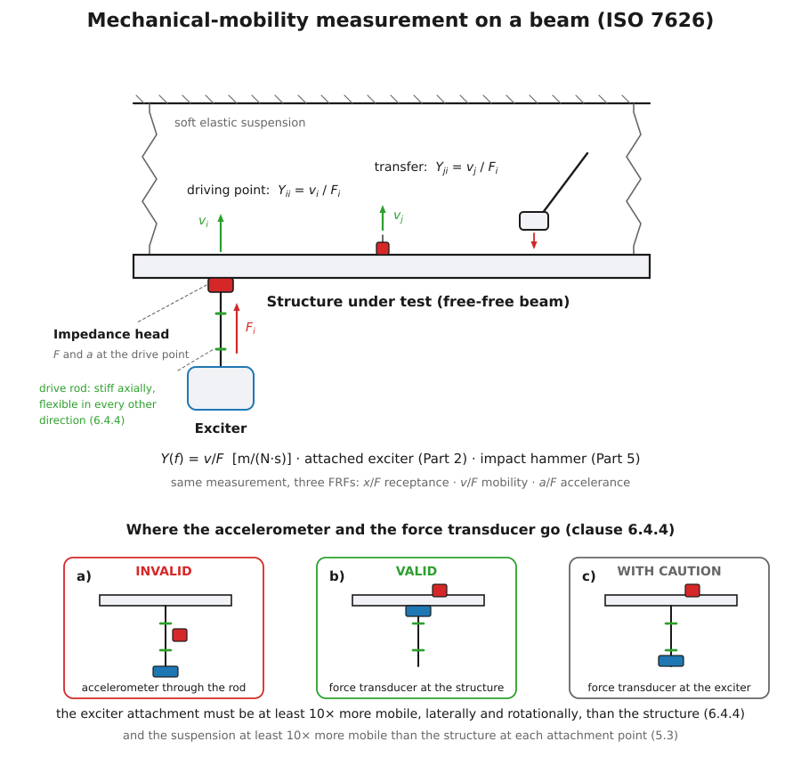
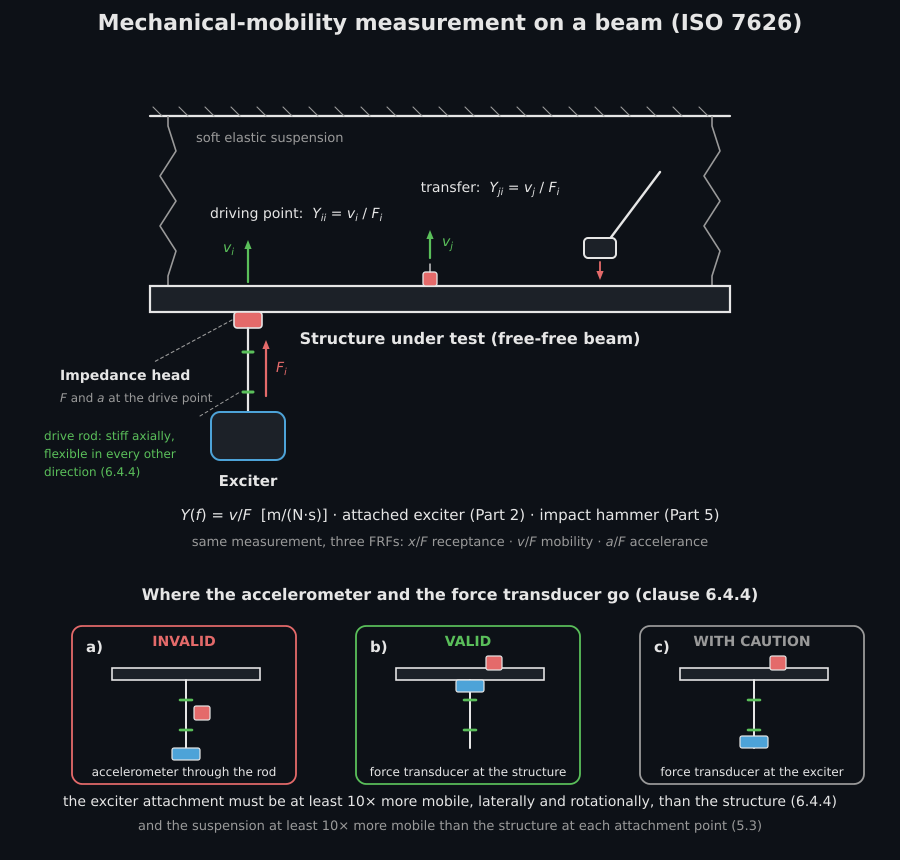
The order of work the part implies, and the function that judges each step:

1. Calibrate on a rigid block of known mass, freely suspended, at the start and end of each series and whenever the tip or the mass changes (7.2). Its accelerance should read $1/m$ within ±5 %: rigid_mass_calibration_check, the ISO 7626-2 check that 7.2 calls essentially the same procedure.
2. Check the channels against each other by feeding one broad-band signal to both: unity within ±5 % and zero phase within ±5° (8.1), verify_channel_match.
3. Set the frequency range and the record. The sample rate is 2.56 to 4 times the filter cut-off (8.3), and the record should be long enough for the response to decay to about 1 % of its start.
4. Strike once at the highest force the test will use and check the channels for saturation (8.4, check_overload) and the force spectrum across the range of interest (6.3, check_force_spectrum). Change the tip or the mass if the pulse is too short or too long.
5. Strike at least five times at the same point, letting the structure come to rest in between (8.6), and discard any record with a double hit (6.4, check_double_hit). Three to five impacts are usually enough to verify data quality in a low-noise environment (8.6), and five is the fewest records a high coherence is trusted from (9.1), which is what the coherence check of step 7 asks for.
6. Judge the decay (8.3, 8.5.2, check_response_decay, given the force so the impact itself is left out), and if it is too slow, add an exponential window and plan to correct for it (Annex A).
7. Average (8.6, impact_mobility) and judge the coherence (9.1, check_coherence).

The analyser samples $N$ points at an interval $\Delta t$, a record of length $T=N\Delta t$ whose discrete Fourier transform has $N/2+1$ lines $1/T$ apart (8.3). When the transient lies wholly inside the record, the transform scaled by $\Delta t$ samples the continuous Fourier transform $F(f)$, and the part describes the pulse by its energy spectral density (3.3, 3.4), the power spectral density $2|F{|}^2/T$ multiplied by the record length:

A pulse has a main lobe at low frequency and side lobes that fall quickly, and its usable bandwidth is inversely proportional to its duration (6.2): a harder tip or a lighter hammer widens it, a softer tip or a heavier hammer narrows it (6.3).

The force typically occupies less than 1 % of the record (8.5.1), and whatever noise the force channel carries runs through all of it. Because the noise adds to the force auto-spectrum, averaging does not remove it. The force window does: unity over the part of the record that holds the pulse and its filter response, exactly zero everywhere else. The noise that reaches the spectrum is then only the noise inside the window.

import numpy as np
from scipy import signal
from phonometry import vibration

fs, n = 4096.0, 4096                      # a 1 s record: 1 Hz between lines
t = np.arange(n) / fs

# A 2 kg resonator tuned to 50 Hz with 0.5 % damping, struck by a 0.5 ms pulse.
m, fn, zeta = 2.0, 50.0, 0.005
wn = 2.0 * np.pi * fn
accelerance = signal.lti([1.0 / m, 0.0, 0.0], [1.0, 2.0 * zeta * wn, wn**2])
force = 100.0 * np.exp(-((t - 0.005) ** 2) / (2.0 * 0.0005**2))
_, accel, _ = signal.lsim(accelerance, force, t)

# The same pulse with broad-band noise on the force channel, and a force
# window that keeps the first 15 ms of the record (8.5.1).
rng = np.random.default_rng(7626)
noisy = force + 0.3 * rng.standard_normal(n)
window = vibration.force_window(n, fs, width_s=0.015)
f, whole = vibration.energy_spectral_density(noisy, fs)
_, kept = vibration.energy_spectral_density(noisy * window, fs)
above = f > 1500.0                        # where the pulse itself has gone
print(round(10 * np.log10(whole[above].mean() / kept[above].mean()), 1))  # 18.4 dB
print(round(10 * np.log10(1.0 / 0.015), 1))    # 18.2 dB, 10 lg(T / width)

The floor drops by the ratio of the record to the window, 18 dB here, and the pulse is untouched because the window never attenuates it. Two warnings come with the window. A rectangular one spreads periodic noise and DC offset over a wide band (8.5.1, Figure 8), so remove those before windowing; taper_s adds half-cosine ramps outside the unity part if a smooth edge is wanted. And it must never cut a second impact out of the record (6.4): the response still carries that impact. impact_mobility warns with ImpactExcitationWarning when its force window zeroes an impact the record holds.

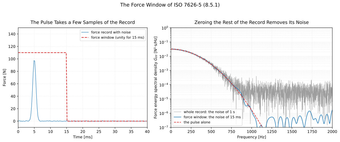
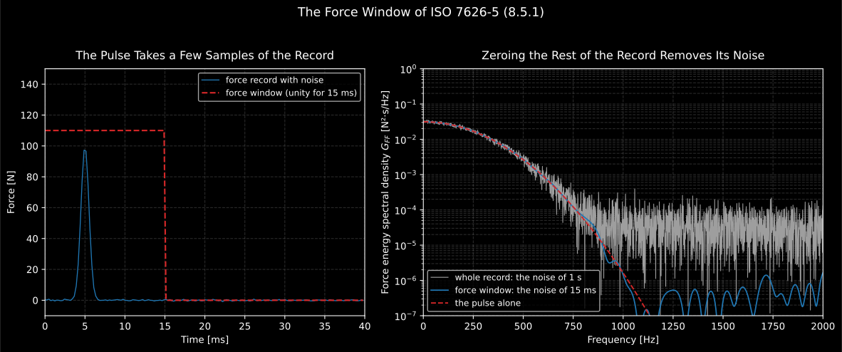
The force window at work. The pulse fills a few samples of the one-second record; everything after 15 ms is noise, and zeroing it lowers the floor of the force spectrum by about 18 dB without changing the pulse’s own spectrum, which is what 8.5.1 means by a window that “introduces no distortion”.

vibration.check_force_spectrum(noisy * window, fs, frequency_range_hz=(0.0, 800.0),
                               max_drop_db=20.0).plot()

import matplotlib.pyplot as plt

fig, (left, right) = plt.subplots(1, 2, figsize=(12.4, 5.2))
shown = t <= 0.04
left.plot(1e3 * t[shown], noisy[shown], label="force record with noise")
left.plot(1e3 * t[shown], 110.0 * window[shown], "--",
          label="force window (unity for 15 ms)")
left.set_xlabel("Time [ms]"); left.set_ylabel("Force [N]"); left.legend()

_, clean = vibration.energy_spectral_density(force, fs)
band = (f > 0.0) & (f <= 2000.0)
right.semilogy(f[band], whole[band], color="0.6", label="whole record")
right.semilogy(f[band], kept[band], label="force window")
right.semilogy(f[band], clean[band], "--", label="the pulse alone")
right.set_ylim(1e-7, 1.0)
right.set_xlabel("Frequency [Hz]"); right.set_ylabel("$G_{FF}$ [N²·s/Hz]")
right.legend(); plt.show()

Averaging over several impacts at one point improves the estimate, and the part prescribes the form: the averaged cross-spectrum of response and force divided by the averaged auto-spectrum of the force (8.6), the H1 estimator, with the ordinary coherence beside it (9.1):

In a low-noise environment three to five impacts are usually enough to verify the data (8.6), and the response must have decayed below the limit of detection before the next impact, or its ringing corrupts the next record.

# Five impacts of different strength, a little noise on the accelerometer.
gains = np.array([0.8, 1.0, 1.1, 0.9, 1.2])[:, np.newaxis]
forces = force * gains
accels = accel * gains + 0.02 * rng.standard_normal((5, n))
estimate = vibration.impact_mobility(forces, accels, fs, force_window_s=0.015,
                                     frequency_range_hz=(5.0, 800.0))
print(estimate.impacts, estimate.measured_frf)     # 5 accelerance

coh = vibration.check_coherence(estimate, frequency_range_hz=(10.0, 400.0))
print(coh.passes, round(float(coh.coherence.min()), 3))   # True 0.992
print(round(float(np.nanmax(coh.random_error_percent)), 2))  # 2.83 %

Each row of forces and accels is one impact. The response channel measured acceleration, so the estimate is formed as an accelerance and converted to mobility (estimate.to(...) gives any other kind). frequency_range_hz keeps it to the frequency range of interest of 3.2: above the usable bandwidth of the pulse the spectrum is noise over almost no force, and nothing built on the result, its plot, its fiche or a fit, should see that part.

Records read from a measurement file arrive as a Signal: pass it in place of the array and leave out fs, which it brings with it (one impact per channel). A force and an acceleration are not pressures, so a calibration factor the Signal carries is not applied to them. The checks of section 5 that read a record take a Signal the same way.

The coherence check passes when ${\gamma }^2$ exceeds 0.9 at every frequency it judges and at least five impacts were averaged. Both numbers are 9.1’s: a coherence above 0.9 is what it calls high, and five to ten records are what a high coherence needs for confidence in its own estimate. Five is also the top of the three to five that 8.6 finds usually enough, so averaging five satisfies both; minimum_records lowers the count when fewer were judged enough. A single impact has a coherence of 1 by construction, which is why it fails the second condition. Low coherence at an antiresonance is not generally a concern (9.1 NOTE 1), and exclude_hz=[(f_low, f_high), ...] leaves such bands out of the verdict. The coherence does not see everything: a repeatable impact hides leakage, structural nonlinearity and clipping (9.1 NOTE 2), which is what the checks of section 5 are for.

The estimate above has a flaw the coherence cannot see:

at_50 = estimate.frequencies == 50.0
print(round(float(estimate.magnitude[at_50][0]), 4))   # 0.1257 m/(N·s)
print(round(1.0 / (2.0 * zeta * m * wn), 4))           # 0.1592, the true peak

The peak is 21 % low. The resonator is so lightly damped that it is still ringing when the one-second record ends, and the transform of a truncated decay leaks. The part’s rule is that the response should decay to about 1 % of its initial magnitude by the end of the record, a figure 8.3 calls a compromise: a longer record improves the frequency resolution but can lower the signal-to-noise ratio. It offers a convenient check too: the peak at the midpoint of the record about 10 % of the highest (8.3, 8.5.2).

# Give the check the force of the same impact: a driving-point acceleration
# follows the force during the impact (the mass line), so the decay is judged
# from the end of the pulse on.
decay = vibration.check_response_decay(accel, fs, force=force)
print(decay.passes, round(100 * decay.end_ratio, 1))    # False 21.1 (%)
print(round(100 * decay.midpoint_ratio, 1))             # 46.3 (%), not 10 %

The level at the end is read at the last sample. The largest value over the last segment of the record sits at the segment’s start, above the end of a decay still under way, so the check carries it to the last sample at the rate the peaks fall from the midpoint to the last segment, the steady decay the midpoint check itself assumes. The verdict compares that level with the printed figure to a whole per cent, so “about 1 %” passes any level below 1.5 %, which rounds to 1 %. Without the force, the highest peak of this record is the impact, two and a half times the free decay, and the same record would read 8.5 %.

A longer record would need a block size or a zoom band the analyser may not have (8.3). The alternative the part recommends is an exponential window, $w(t)={\mathrm{e}}^{-at}$, which starts at unity and adds a known decay to the data so the record ends where it should. As a general guideline, the natural decay should still reach 25 % or less within the record, or the correction of Annex A becomes too sensitive to errors in the damping estimate (8.5.2), and the check applies that limit when told a window will be used:

windowed_decay = vibration.check_response_decay(accel, fs, force=force,
                                                exponential_window=True)
print(windowed_decay.passes, windowed_decay.limit_ratio)   # True 0.25

rate = vibration.exponential_decay_rate(n, fs, final_value=0.01)
print(round(rate, 3))                                      # 4.606 1/s
windowed = vibration.impact_mobility(forces, accels, fs, force_window_s=0.015,
                                     exponential_decay_rate_per_s=rate,
                                     frequency_range_hz=(5.0, 800.0))
print(round(float(windowed.magnitude[at_50][0]), 4))       # 0.0404 m/(N·s)

The window traded one error for another. The leakage is gone, but the peak is now a quarter of the true one: the window multiplies the whole response by a decay, and a mode that decays faster looks more damped. That is not a mistake to be avoided but a known quantity to be taken out, which is what Annex A does.

Multiply both sides of the convolution $x(t)={\int }_0^{t}h(\tau )f(t-\tau )\mathrm{d}\tau$ (Formula (A.1)) by ${\mathrm{e}}^{-at}$, and because ${\mathrm{e}}^{-at}={\mathrm{e}}^{-a\tau }{\mathrm{e}}^{-a(t-\tau )}$ the windowed response is the windowed force convolved with a windowed impulse response (Formula (A.2)). Every mode $A_r{\mathrm{e}}^{s_{r}t}$ of the impulse response becomes $A_r{\mathrm{e}}^{(s_r-a)t}$: the window moves each pole back by $a$ and leaves its residue alone. A damping ratio ${\hat{\zeta }}_r$ estimated from windowed data therefore carries the window’s share, and Formula (A.3) removes it:

with ${\omega }_r$ the damped natural frequency in rad/s. For a lightly damped, well separated mode the measured peak is multiplied by ${\hat{\zeta }}_r/{\zeta }_r$ to give the true one.

The annex leaves the damping estimator open (“a variety of curve-fitting methods”), and single_mode_fit is the one this library offers: a rational-fraction fit of one mode over a band, written as a pole, its residue and a constant for the modes outside the band. ImpactMobilityResult.fit_mode runs it on the kind the response channel measured, the record the window actually multiplied, and remembers the window’s rate:

fit = windowed.fit_mode((40.0, 60.0))
print(round(fit.damped_natural_frequency_hz, 2))             # 50.0 Hz
print(round(100 * fit.apparent_damping_ratio, 3))            # 1.966 %

correction = fit.correction
print(round(100 * float(correction.window_damping_ratio[0]), 3))  # 1.466 %, a / omega_r
print(round(100 * float(correction.damping_ratio[0]), 3))         # 0.499 %, Formula (A.3)
print(round(100 * float(correction.exact_damping_ratio[0]), 3))   # 0.5 %, the pole moved back
print(round(float(correction.peak_correction_factor[0]), 2))      # 3.94

f_d = fn * np.sqrt(1.0 - zeta**2)
print(round(abs(complex(fit.corrected_mobility(f_d))), 4))   # 0.1588 m/(N·s)

The damping comes back as 0.499 % against a true 0.5 %, and the synthesized mobility, the fitted mode with its pole moved back by $a$, peaks at 0.1588 against the true 0.1592. What is left, about 0.2 %, is truncation again: the windowed record still ends at about 0.2 % of its start, 21 % of natural decay times 1 % of window.

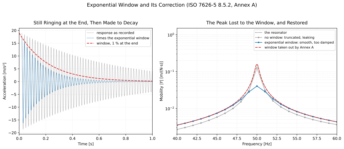
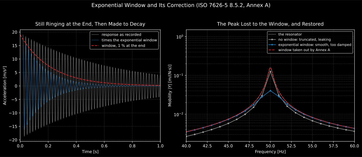
What the window takes and what Annex A gives back. Unwindowed, the estimate leaks: it is low at the peak and low on the flanks by an amount no correction can predict (8.5.2). Windowed, it is smooth but too damped, by an amount that is known, and moving the fitted pole back by $a$ lands on the resonator.

fit.plot()

import matplotlib.pyplot as plt

fig, (left, right) = plt.subplots(1, 2, figsize=(12.4, 5.4))
w = vibration.exponential_window(n, fs, decay_rate_per_s=rate)
free = t >= 0.02
left.plot(t[free], accel[free], color="0.6", lw=0.6, label="response as recorded")
left.plot(t[free], (accel * w)[free], lw=0.6, label="times the exponential window")
left.plot(t, float(np.max(np.abs(accel[free]))) * w, "--", label="window, 1 % at the end")
left.set_xlabel("Time [s]"); left.set_ylabel("Acceleration [m/s²]"); left.legend()

single = vibration.impact_mobility(force, accel, fs, frequency_range_hz=(5.0, 800.0))
single_windowed = vibration.impact_mobility(force, accel, fs,
                                            exponential_decay_rate_per_s=rate,
                                            frequency_range_hz=(5.0, 800.0))
dense = np.linspace(40.0, 60.0, 2001)
band = (single.frequencies >= 40.0) & (single.frequencies <= 60.0)
exact = vibration.sdof_mobility(dense, m, m * wn**2, 2.0 * zeta * m * wn)
right.semilogy(dense, np.abs(exact), "k:", label="the resonator")
right.semilogy(single.frequencies[band], single.magnitude[band], "o-", color="0.6",
               label="no window: truncated, leaking")
right.semilogy(single_windowed.frequencies[band], single_windowed.magnitude[band],
               "o-", label="exponential window: smooth, too damped")
single_fit = single_windowed.fit_mode((40.0, 60.0))
right.semilogy(dense, np.abs(single_fit.corrected_mobility(dense)), "--",
               label="window taken out by Annex A")
right.set_xlabel("Frequency [Hz]"); right.set_ylabel("Mobility |Y| [m/(N·s)]")
right.legend(); plt.show()

The annex states the effect exactly, the pole replaced by $s_r-a$, and then gives (A.3) for the damping. The two are not the same thing. The windowed pole has the decay rate ${\hat{\sigma }}_r={\sigma }_r+a$ at the same damped frequency ${\omega }_r$, and a damping ratio is a decay rate over the undamped frequency, $\zeta =\sigma /\sqrt{{\sigma }^2+{\omega }_r^2}$, which moves with the decay rate. Solving that exactly and expanding gives (A.3) plus a remainder of about $({\hat{\zeta }}_r^3-{\zeta }_r^3)/2$, always on the low side. The result carries both: damping_ratio is (A.3) as printed and exact_damping_ratio is the damping of the pole moved back, which is also what corrected_frf and corrected_mobility synthesize.

The difference is invisible with the window of the example, which adds 1.5 % of damping, and grows quickly with a heavier one:

heavy = vibration.impact_mobility(forces, accels, fs, force_window_s=0.015,
                                  exponential_decay_rate_per_s=20.0,
                                  frequency_range_hz=(5.0, 800.0))
heavy_correction = heavy.fit_mode((40.0, 60.0)).correction
print(round(100 * float(heavy_correction.apparent_damping_ratio[0]), 3))  # 6.851 %
print(round(100 * float(heavy_correction.damping_ratio[0]), 3))           # 0.484 %
print(round(100 * float(heavy_correction.exact_damping_ratio[0]), 3))     # 0.5 %

This is not a misprint. The annex writes (A.3) for a “damping factor” it does not define, and the part takes its terms from ISO 2041 (clause 3), whose damping ratio is the damping coefficient over the critical one, $c/c_c$ (ISO 2041:2018, 3.2.96). For that ratio (A.3) is the first order of the pole shift; for a decay rate over the damped frequency, ${\sigma }_r/{\omega }_r$, it would be exact. It is a reason to keep the window light, the same advice 8.5.2 gives for another reason, and to prefer the exact form when the window adds several per cent.

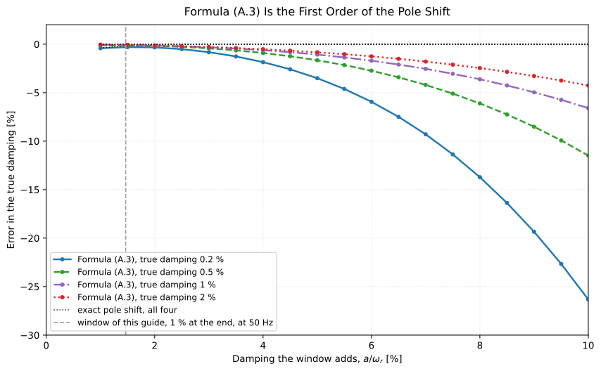
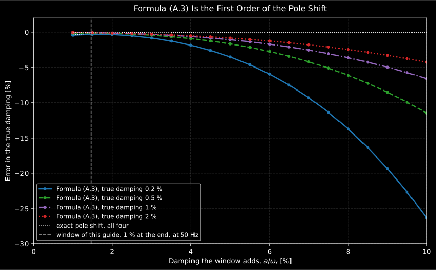
Formula (A.3) against the exact pole shift, each point a full measurement: the resonator struck, windowed, fitted and corrected. The lighter the structure, the sooner (A.3) falls behind, because the window’s damping then dominates the apparent damping the formula starts from.

fit.correction.plot()

import matplotlib.pyplot as plt

ratios = np.linspace(0.01, 0.1, 19)
omega_d = 2.0 * np.pi * fn
for true in (0.002, 0.005, 0.01, 0.02):
    w_n = omega_d / np.sqrt(1.0 - true**2)
    system = signal.lti([1.0 / m, 0.0, 0.0], [1.0, 2.0 * true * w_n, w_n**2])
    _, response, _ = signal.lsim(system, force, t)
    a3, exact = [], []
    for ratio in ratios:
        result = vibration.impact_mobility(force, response, fs,
                                           exponential_decay_rate_per_s=ratio * omega_d,
                                           frequency_range_hz=(5.0, 800.0))
        c = result.fit_mode((40.0, 60.0)).correction
        a3.append(float(c.damping_ratio[0]))
        exact.append(float(c.exact_damping_ratio[0]))
    plt.plot(100 * ratios, 100 * (np.array(a3) - true) / true, "o-",
             label=f"Formula (A.3), true damping {100 * true:g} %")
    plt.plot(100 * ratios, 100 * (np.array(exact) - true) / true, "k:")
plt.xlabel(r"Damping the window adds, $a/\omega_r$ [%]")
plt.ylabel("Error in the true damping [%]")
plt.legend(); plt.show()

Two practical points close the annex. The window is often applied to the response alone: the pulse is so short that windowing it amounts to multiplying the force by the window’s value at its peak, which exponential_on_force=False does, and which is close to 1 when the pulse sits near the start of the record. And if the calibration of 7.2 uses the same window and pre-trigger as the measurement, that factor is already in the calibration.

Every check returns a verdict object with passes and a .plot(); reading one as a truth value raises, so a verdict is never mistaken for a number.

Double hits (6.4). Two impacts in one record are two pulses whose transforms interfere: a second pulse $r$ times the first and $\tau$ later multiplies the spectrum by $1+r{\mathrm{e}}^{-j\omega \tau }$, which ripples between $(1+r{)}^2$ and $(1-r{)}^2$ every $1/\tau$ hertz. The notches are deep only when the second impact is about as strong as the first, which is why the part says a small second impact shows as a slight ripple and moderate dips may be tolerated. At a notch there is almost no force, and the mobility there is noise.

double = force + 0.6 * np.roll(force, round(0.06 * fs))   # 60 % again, 60 ms later
hit = vibration.check_double_hit(double, fs)
print(hit.passes, hit.impacts, round(hit.delay_s, 3))     # False 2 0.06
print(round(hit.notch_spacing_hz, 1), round(hit.ripple_db, 1))  # 16.7 12.0
print(vibration.check_double_hit(force, fs).passes)       # True

An impact is a run of samples above a fraction of the largest force, 0.1 by default (threshold_ratio); that number is this library’s, since the part gives none. At 0.1 an undetected second pulse of the same shape as the first ripples the spectrum by at most 1.74 dB. A softer, longer rebound, the usual hammer bounce, carries more of the low-frequency spectrum than its peak says, and can stay under the threshold while it ripples the spectrum by several decibels, which is why 6.4 finds multiple impacts most easily in the frequency domain, where the force-spectrum check below reads them. Run the check on the unwindowed force, and on the unfiltered one when the analyser offers it: the anti-aliasing filter can hide a small second impact in the ringing of the first, which is why 6.4 recommends a storage oscilloscope on the unfiltered signal, and a steep filter can ring above the threshold itself, so that one impact reads as several.

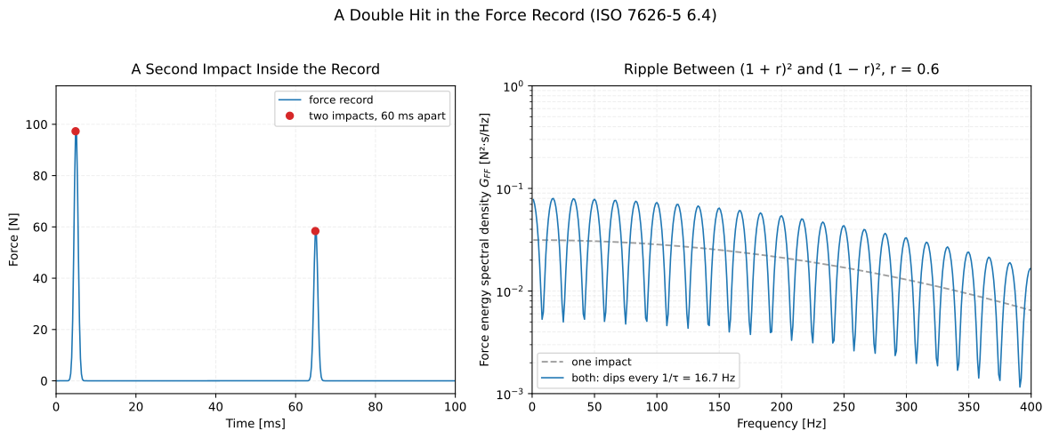
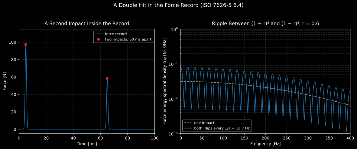
A double hit in the force record. The two impacts are 60 ms apart, so the spectrum dips every 16.7 Hz; with the second at 60 % of the first, it swings between 2.56 and 0.16 times the single pulse’s, 12 dB peak to notch.

hit.plot()

import matplotlib.pyplot as plt

fig, (left, right) = plt.subplots(1, 2, figsize=(12.4, 5.2))
shown = t <= 0.1
left.plot(1e3 * t[shown], double[shown], label="force record")
left.plot(1e3 * hit.impact_times_s, hit.impact_peaks, "o",
          label="two impacts, 60 ms apart")
left.set_xlabel("Time [ms]"); left.set_ylabel("Force [N]"); left.legend()

_, one = vibration.energy_spectral_density(force, fs)
_, both = vibration.energy_spectral_density(double, fs)
band = (f > 0.0) & (f <= 400.0)
right.semilogy(f[band], one[band], "--", color="0.6", label="one impact")
right.semilogy(f[band], both[band], label="both: dips every 16.7 Hz")
right.set_xlabel("Frequency [Hz]"); right.set_ylabel("$G_{FF}$ [N²·s/Hz]")
right.legend(); plt.show()

The force spectrum (6.2, 6.3). The pulse should put its energy into the frequency range of interest and not far beyond it. The check reads how far the energy spectral density falls across the range, from its highest to its lowest value there, against a limit the caller states, because the part prints none; beside it, the share of the force energy above the range, which 6.3 asks to keep small:

spectrum = vibration.check_force_spectrum(force, fs, frequency_range_hz=(0.0, 400.0),
                                          max_drop_db=10.0)
print(spectrum.passes, round(spectrum.drop_db, 2))       # True 6.86 (dB)
print(round(100 * spectrum.energy_fraction_above, 1))    # 7.5 % above 400 Hz

wide = vibration.check_force_spectrum(force, fs, frequency_range_hz=(0.0, 1000.0),
                                      max_drop_db=10.0)
print(wide.passes, round(wide.drop_db, 1))               # False 42.9: a harder tip

A double hit fails the same check through its notches (18.4 dB across 0 to 400 Hz for the record above), which is the part’s own advice: multiple impacts are most easily detected in the frequency domain (6.4).

Overload (8.4). Impact signals carry energy out of band, and the dynamic range is used to its limit, so saturation is a real risk. The check compares each channel with the manufacturer’s maximum for linear operation; a pass is necessary, not sufficient, because a filtered digital record gives poor definition of the waveform the converter saw:

over = vibration.check_overload(accel, fs, full_scale=50.0)
print(over.passes, round(over.peak, 1), round(over.headroom_db, 1))   # True 47.6 0.4

Channel match (8.1). One broad-band signal into both channels, the frequency response between them estimated, for instance with phonometry.electroacoustics.frequency_response.transfer_function, and verify_channel_match(frequencies, response, frequency_range_hz=...) asks for unity within ±5 % and zero phase within ±5° across the range. It is the one check here that judges the instrument rather than the record, hence verify_ rather than check_.

Calibration (7.2). The rigid-block check of ISO 7626-2 7.5.2, rigid_mass_calibration_check, described on the mobility page. The block’s mass shall be chosen so its mobility is representative of the mobilities to be measured, and the hammer and the analyser shall be set up exactly as in the measurement.

ImpactMobilityResult.report(path) renders the one-page ISO 7626 fiche with the basis line naming ISO 7626-5:2019 and the averaging of 8.6, and the table extended by the number of impacts, the exponential window and the coherence at the peak. When a window was used, the fiche says the peaks carry its damping: the corrected mobility is a modal result, and the fiche reports the measurement.

from phonometry import ReportMetadata

windowed.report(
    "impact_mobility.pdf",
    metadata=ReportMetadata(
        specimen="Machine support bracket (driving point)",
        measurement_standard="ISO 7626-5",
    ),
)   # one-page fiche (needs phonometry[report,plot])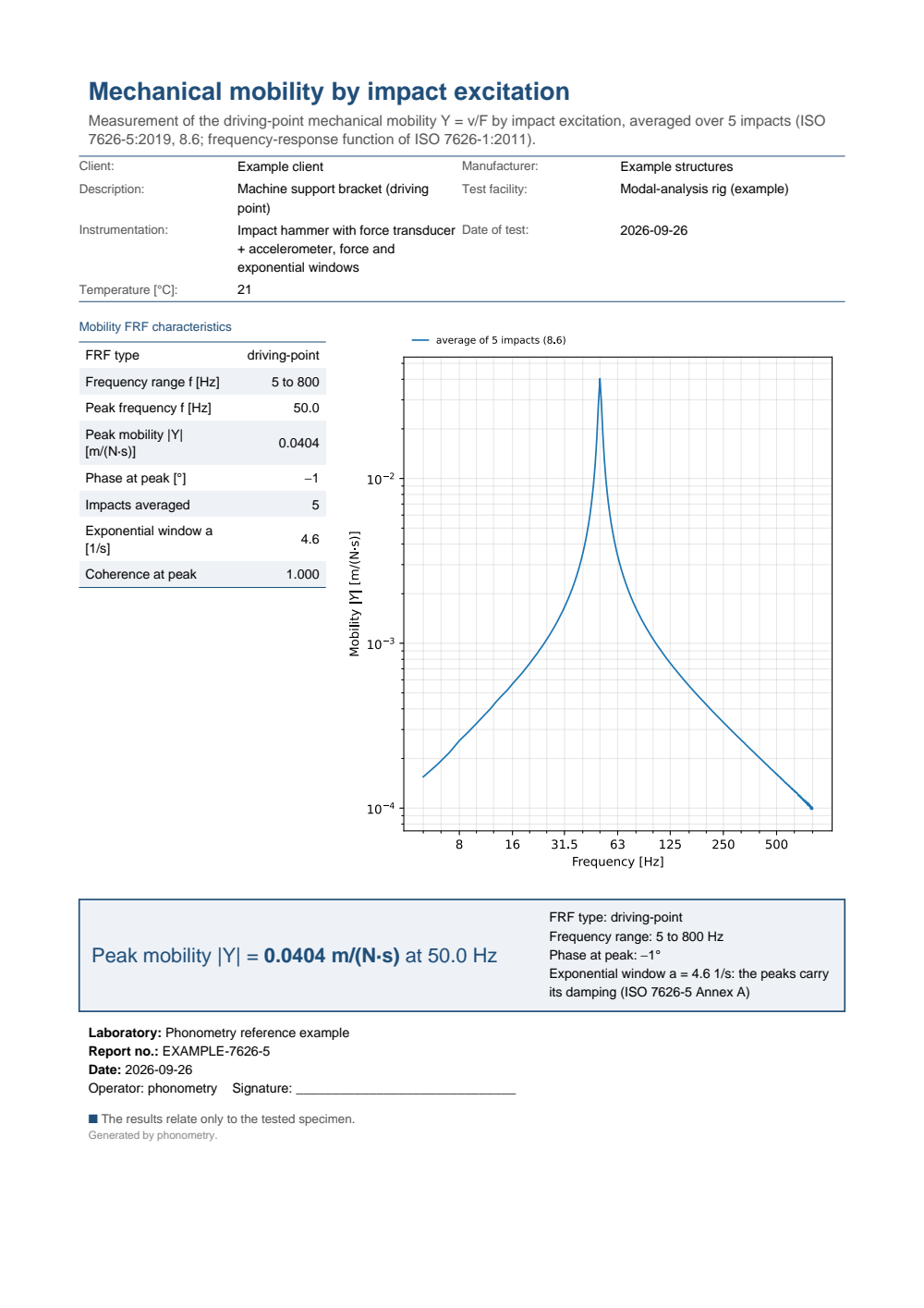

One-page mechanical-mobility fiche for an impact measurement: a metadata header, a table of the characteristic points (the FRF type, the frequency range of 5 to 800 hertz, the peak at 50 hertz, the peak mobility of 0.0404, the phase there, five impacts averaged, an exponential window of 4.6 per second and a coherence of 1.000 at the peak) beside the averaged mobility spectrum, and the boxed peak mobility with a note that the peaks carry the window's damping.

Download the report (PDF)

• Covered

  ISO 7626-5:2019’s processing of impact records: the energy spectral density of 3.3 and 3.4 (energy_spectral_density), the force window of 8.5.1 (force_window), the exponential window of 8.5.2 (exponential_window, exponential_decay_rate), the averaged H1 estimate over impacts of 8.6 with the coherence of 9.1 (impact_mobility, ImpactMobilityResult), the damping correction of Annex A both as Formula (A.3) and as the exact pole shift (exponential_window_correction), with a single-mode rational-fraction fit to estimate the damping (single_mode_fit, ImpactMobilityResult.fit_mode), and the verdicts on the record: double hits (6.4), the force spectrum across the range of interest (6.2, 6.3), overload (8.4), the response decay (8.3, 8.5.2), the coherence (9.1) and the channel-to-channel match of the analyser (8.1). The calibration of 7.2 runs through the ISO 7626-2 rigid-mass check.

• Not covered

  The part’s guidance on hardware is described, not computed: the choice of tip and impactor mass (6.1, 6.3), the 10° alignment of the impact (6.1), the suspension of clause 5 and the alias-protection test of 8.1. The limits of the force-spectrum check and the double-hit threshold are the caller’s and the library’s, because the part prints none. The single-mode fit is one estimator among many and needs a band with one resonance in it: closely spaced modes need a multi-mode curve fitter, which is not provided, and zoom analysis (8.3 b) is not implemented. The repeatability, reciprocity, linearity and attached-exciter comparisons of 9.2 to 9.5 are left to the operator.

References

Section titled “References”- International Organization for Standardization. (2011). Mechanical vibration and shock — Experimental determination of mechanical mobility — Part 1: Basic terms and definitions, and transducer specifications (ISO 7626-1:2011). The FRF family (Table 1) the estimate is expressed in: accelerance from an accelerometer, converted to mobility.
- International Organization for Standardization. (2015). Mechanical vibration and shock — Experimental determination of mechanical mobility — Part 2: Measurements using single-point translation excitation with an attached vibration exciter (ISO 7626-2:2015). The operational calibration on a rigid mass of 7.5.2, which ISO 7626-5 7.2 calls essentially the same procedure, and the random-error formula of Annex A that the coherence check reports.
- International Organization for Standardization. (2018). Mechanical vibration, shock and condition monitoring — Vocabulary (ISO 2041:2018). The damping ratio, the damping coefficient over the critical one (3.2.96), against which Formula (A.3) is first order; ISO 7626-5 takes its terms from it (clause 3).
- International Organization for Standardization. (2019). Mechanical vibration and shock — Experimental determination of mechanical mobility — Part 5: Measurements using impact excitation with an exciter which is not attached to the structure (ISO 7626-5:2019). The whole page: the energy spectral density of 3.3 and 3.4, the double hits of 6.4, the calibration of 7.2, the channel match of 8.1, the sampling and decay rules of 8.3, saturation (8.4), the force window of 8.5.1, the exponential window of 8.5.2, the averaging of 8.6, the coherence of 9.1 and the correction of Annex A, Formulas (A.1) to (A.3). It prints no worked example, so conformance is anchored on closed forms: a resonator struck by a Gaussian pulse, whose response is known exactly, gives its mobility and its damping back.