Source: https://docs.jmrp.io/phonometry/start/getting-started/
# Getting Started
## Installation
**Option 1: From PyPI (Recommended)**
```bash
pip install phonometry
```
phonometry needs Python 3.12 or newer, with NumPy 2.0.2 and SciPy 1.14.0
or later. Each of those floors, and each floor of the extras, is the oldest
release the library's tests pass with, and a CI job installs exactly those
releases on Python 3.12 to keep it so: matplotlib 3.10.7 for `[plot]`,
reportlab 4.0.4 and svglib 0.9.0 for `[report]`, numba 0.60.0 for `[perf]` and
python-soundfile 0.12.0 for `[audio]`.
Optional extras:
```bash
pip install phonometry[plot] # matplotlib, for filter response plots and result .plot() methods
pip install phonometry[perf] # numba, faster 'impulse' time weighting
pip install phonometry[report] # reportlab + svglib, so result .report() methods render normative PDF fiches (their figure panel needs [plot] too)
pip install phonometry[audio] # python-soundfile, so phonometry.io also reads FLAC, AIFF, Ogg/Opus, MP3 and compressed WAV
pip install phonometry[full] # all of the above (recommended)
```
I recommend `pip install phonometry[full]`: it brings matplotlib, numba,
reportlab, svglib and soundfile in one go, so every feature of the library is
enabled. The base install computes every metric on NumPy and SciPy alone, and
that includes reading every linear measurement WAV (24-bit, multichannel
EXTENSIBLE, RF64) through `phonometry.io`; the only things it leaves
unavailable are the figures (`.plot()` and the filter response plots), the
normative PDF fiches (`.report()`), the compiled kernel that speeds up the
`impulse` time weighting, and the compressed audio formats. One licensing note
on `[audio]`: it installs python-soundfile, whose wheel bundles **libsndfile
under the LGPL-2.1** (dynamically linked, the same pattern as librosa and
torchaudio). The base install deliberately stays free of it, which is why the
metrological formats need no extra.
One caveat about `[full]`: numba is the only extra that caps NumPy, and it
raises that cap only once it supports a new NumPy minor. So in the weeks after
a NumPy minor release, `phonometry[full]` (like `phonometry[perf]`) can resolve
one minor behind what a plain install gets. numba only makes the `impulse` time
weighting faster, so if you need the newest NumPy the day it ships, install
`phonometry[plot,report]` and leave `[perf]` out.
**Option 2: Cloning and Installing**
```bash
git clone https://github.com/jmrplens/phonometry.git
cd phonometry
pip install .
```
**Option 3: Git Submodule**
```bash
git submodule add https://github.com/jmrplens/phonometry.git
# Then install in editable mode to use it from your project
pip install -e ./phonometry
```
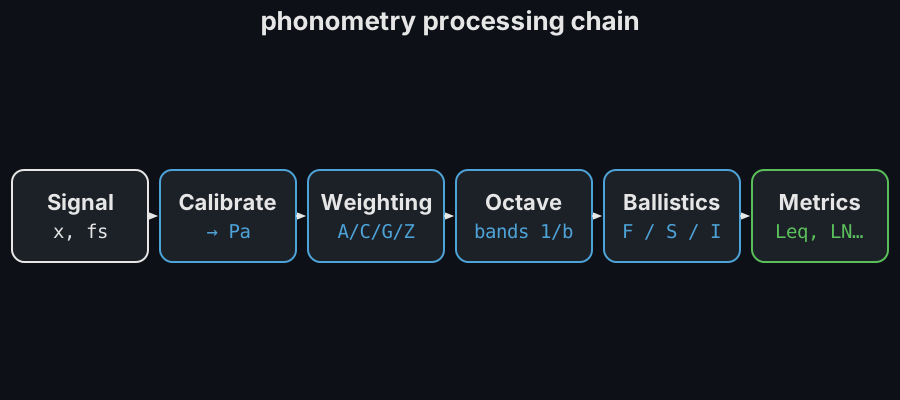
## The processing chain at a glance
Every phonometry analysis is some subset of one pipeline: take the raw
signal, convert it to physical units, weight it in frequency, split it into
standardized bands, smooth it in time and reduce it to metrics:
Each stage is an independent function or class you can use on its own; the
guides cover them left to right ([Calibration](https://docs.jmrp.io/phonometry/signals/metrology/calibration/) →
[Frequency Weighting](https://docs.jmrp.io/phonometry/signals/levels/weighting/) → [Filter Banks](https://docs.jmrp.io/phonometry/signals/filters/filter-banks/) →
[Time Weighting](https://docs.jmrp.io/phonometry/signals/levels/time-weighting/) → [Levels](https://docs.jmrp.io/phonometry/signals/levels/levels/)).
## Basic Usage: 1/3 Octave Analysis
Analyze a signal and get the Sound Pressure Level (SPL) per frequency band.
```python
import numpy as np
from phonometry import filters
fs = 48000
t = np.linspace(0, 1, fs, endpoint=False)
# Composite signal: 100Hz + 1000Hz
signal = np.sin(2 * np.pi * 100 * t) + np.sin(2 * np.pi * 1000 * t)
# Apply 1/3 octave filter bank
result = filters.octave_filter(signal, fs=fs, fraction=3)
print(f"Bands: {result.frequencies}")
# Bands: [12.589254117941678, 15.848931924611138, ..., 19952.623149688785] (33 bands)
print(f"SPL [dB]: {result.levels}")
# SPL [dB]: [46.88395351 47.96774897 49.04991279 ...] — ~90.7 dB at 100 Hz and ~90.9 dB at 1 kHz
```
*Example of a 1/3 Octave Band spectrum analysis of a complex signal.*
Show the code for this figure
```python
import matplotlib.pyplot as plt
import scipy.signal
import numpy as np
from phonometry import filters
fs = 48000
t = np.linspace(0, 1, fs, endpoint=False)
# Composite signal: 100Hz + 1000Hz
signal = np.sin(2 * np.pi * 100 * t) + np.sin(2 * np.pi * 1000 * t)
# Apply 1/3 octave filter bank
filtered = filters.octave_filter(signal, fs=fs, fraction=3)
spl, freq = filtered.levels, filtered.frequencies
# Gray background: the raw-signal PSD (Welch), shifted to sit just below the
# band SPLs so both spectral shapes share one axis.
f_psd, psd = scipy.signal.welch(signal, fs, nperseg=8192)
psd_db = 10 * np.log10(psd + 1e-12)
psd_db += np.max(spl) - np.max(psd_db) - 5
fig, ax = plt.subplots()
ax.semilogx(f_psd, psd_db, color="gray", alpha=0.6, label="Raw signal PSD")
ax.semilogx(freq, spl, marker="o", markerfacecolor="white",
label="1/3 octave bands")
ax.set_xlabel("Frequency [Hz]")
ax.set_ylabel("SPL [dB]")
ax.legend()
plt.show()
```
## Read a sound level meter WAV
With a real meter you have two WAVs: the calibrator take and the
measurement. `phonometry.io` reads both as measurements: native rate
kept, integer PCM scaled exactly to full scale, channels first, nothing
normalized. The `Signal` it returns carries the sample rate and, once you
attach it, the calibration, so the level functions stop asking you to
repeat either:
```python
import numpy as np
from phonometry import io, metrology, signals
# Both files come from the meter, in this order, through one untouched chain.
cal_take = io.read("calibrator.wav") # the 94 dB calibrator tone
cal = metrology.sensitivity(np.asarray(cal_take), target_spl=94.0,
fs=cal_take.fs)
sig = io.read("measurement.wav", calibration_factor=cal)
print(f"Leq = {float(signals.leq(sig)):.1f} dB") # no fs, no factor to repeat
```
The base install reads everything a meter writes: 24-bit PCM, multichannel
EXTENSIBLE, overnight RF64. It warns if the file is a compressed listening
copy rather than a linear recording. Write the factor into the sidecar once
(`io.write_sidecar("measurement.wav", cal)`) and from then on
`io.read("measurement.wav")` comes back calibrated with no arguments at all.
[Reading and writing measurement audio](https://docs.jmrp.io/phonometry/io/audio-files/) is the full
workflow: provenance, streaming, BWF writing and lossless conversion.
## Analyzing an audio file
```python
from scipy.io import wavfile
from phonometry import filters
# Load standard WAV file
fs, signal = wavfile.read("measurement.wav")
# Analyze
# Note: To obtain real-world SPL values, you must calibrate the input.
# See the Calibration guide.
filtered = filters.octave_filter(signal, fs=fs, fraction=3)
spl, freq = filtered.levels, filtered.frequencies
```
Integer audio (e.g. int16 WAV data) is converted to float64 internally, so it
is safe to pass `wavfile.read` output directly, but note it is *cast*, not
rescaled to full scale, so keep calibrator and measurement in the same format;
`io.read` in the previous section scales exactly and removes the concern.
## In a notebook
Jupyter, JupyterLab, VS Code and Colab display the value of the last line of a
cell, and a result displays as a table of its fields: each with its unit when
its name carries one (`_db`, `_hz`, `_m`...), each array as one line with its
shape and the range of its values, never the values themselves, so the frames
of a simulation take a single row. A verdict shows its outcome, PASS or FAIL,
in the title. Showing the table reads the fields and, on a verdict, `passes`,
which may read other properties of the verdict; it draws nothing and runs
nothing else. `print()` and `repr()` are unchanged: the dataclass repr, with
numpy's own summary of an array longer than a thousand values.
This cell filters a 1 kHz tone over noise into one-third-octave bands and ends
in the result:
```python
import numpy as np
from phonometry import building, filters
fs = 48000
t = np.arange(fs) / fs
rng = np.random.default_rng(7)
noise = np.cumsum(rng.standard_normal(fs))
noise /= np.std(noise)
x = 0.4 * np.sin(2 * np.pi * 1000.0 * t) + 0.05 * noise
bank = filters.octave_filter(x, fs, fraction=3, limits=[20.0, 20000.0])
bank # the last line of the cell: the notebook shows its table
```
Jupyter shows it under the cell as this table:
OctaveFilterResult
field
value
unit
levels
array 31 float64, 17.125 to 82.986
frequencies
list of 31 numbers, 19.953 to 19953
bands
None
plot()
A verdict, in a cell of its own, shows its outcome in the title. This one
applies Annex G.4 of ISO 10140-1 to a [lining test](https://docs.jmrp.io/phonometry/buildings/insulation/lab-application-rules/) on a masonry wall:
the measurements without and with the lining may be a day apart only once the
wall has cured for two weeks, or for at least three times that lag, and
2.9 days is neither:
```python
check = building.check_lining_curing(curing_time_days=2.9, time_lag_days=1.0)
check # a verdict: its outcome in the title
```
LiningCuringCheckFAIL
field
value
unit
curing_time_days
2.9
d
time_lag_days
1
d
required_curing_days
14
d
plot()
The IPython terminal prints the same tables as text:
```text
OctaveFilterResult
levels array 31 float64, 17.125 to 82.986
frequencies list of 31 numbers, 19.953 to 19953
bands None
plot()
LiningCuringCheck: FAIL
curing_time_days 2.9 d
time_lag_days 1 d
required_curing_days 14 d
plot()
```
The last line names what the result can draw. `.plot()` returns the
matplotlib axes, and a notebook draws the figure under the cell with its
inline backend, with no `plt.show()`; in a script, call `plt.show()` or save
the figure:
```python
ax = bank.plot() # drawn under the cell; in a script, plt.show()
```
*The figure `bank.plot()` draws under the cell: the one-third-octave spectrum
of the 1 kHz tone over noise.*
## Where to go next
The octave analysis above uses the `filters` core, one of twenty-one domain
namespaces; the documentation index walks through the rest, from
psychoacoustics and room, building and vibration acoustics to environmental,
aircraft and underwater noise, electroacoustics and FDTD wave simulation.
Every result object exposes a one-line `.plot(language="en"|"es")` figure and,
where a standard defines a reporting format, a `.report()` method that renders
the normative PDF fiche.
- [Filter Architecture Gallery](https://docs.jmrp.io/phonometry/signals/filters/filter-gallery/): choose an architecture and inspect responses
- [Calibration and dBFS](https://docs.jmrp.io/phonometry/signals/metrology/calibration/): get real-world SPL values
- [Why phonometry](https://docs.jmrp.io/phonometry/start/why-phonometry/): the conformance-first design philosophy
- [Conformance report](https://docs.jmrp.io/phonometry/reference/conformance/): the expected and computed value of all 1893 checks
- [API Reference](https://docs.jmrp.io/phonometry/reference/api/): every parameter of every function
- [Bibliography](https://docs.jmrp.io/phonometry/reference/bibliography/): the books and papers behind every guide, each with a verified link