Source: https://docs.jmrp.io/phonometry/reference/theory/signal-analysis/ # Theory: Signal Analysis This page collects the theory behind the measurement chain itself: the standardized fractional-octave bands and the time-domain filter banks that implement them, the frequency weighting curves, time integration, level, event and exposure metrics, sound intensity, and the GUM uncertainty framework that underpins every measured quantity. It is part of the [theory reference](https://docs.jmrp.io/phonometry/reference/theory/). ## Octave Band Frequencies (ANSI S1.11 / IEC 61260) The mid-band frequencies ($f_\mathrm{m}$) and edges ($f_1$, $f_2$) use a base-10 ratio: $$ G = 10^{0.3} $$ **Mid-band:** $$ f_\mathrm{m} = 1000 \cdot G^{x/b} $$ (for odd $b$) **Band edges:** $$ f_1 = f_\mathrm{m} \cdot G^{-1/(2b)}, \quad f_2 = f_\mathrm{m} \cdot G^{1/(2b)} $$ ## Frequency Resolution vs FFT Bin Spacing `octave_filter` is a **time-domain fractional-octave filter bank**, not an FFT or Welch spectrum estimator. Therefore, its result does not have a frequency resolution in the `fs / nfft` sense. For `fraction=3`, the output contains one scalar level per third-octave band. The relevant frequency granularity is the standardized band definition: center frequency, lower edge, and upper edge. Because fractional-octave bands are logarithmically spaced, their absolute bandwidth in Hz grows with frequency while their relative bandwidth remains approximately constant. For example, with `fraction=3` and `limits=[12, 20000]`, the exact third-octave band around 1 kHz is approximately: | Nominal band | Lower edge | Center | Upper edge | Bandwidth | | :--- | ---: | ---: | ---: | ---: | | 1 kHz | 891.25 Hz | 1000.00 Hz | 1122.02 Hz | 230.77 Hz | You can inspect the exact bands with: ```python from phonometry import filters fc, fl, fu, labels = filters.nominal_frequencies(fraction=3, limits=[12, 20000]) for label, center, lower, upper in zip(labels, fc, fl, fu): print(label, center, lower, upper, upper - lower) ``` If you need narrowband FFT bins for tonal inspection, run Welch/FFT on the original signal and use the phonometry band edges as masks: ```python import numpy as np from scipy import signal from phonometry import filters fs = 100_000 # any 1D pressure signal in Pa (synthesized here so the example runs) pressure_signal_pa = 0.02 * np.random.default_rng(0).standard_normal(fs) x = pressure_signal_pa # Standardized third-octave levels from phonometry. filtered = filters.octave_filter( x, fs=fs, fraction=3, limits=[12, 20_000], ) levels, centers = filtered.levels, filtered.frequencies # Same standardized band definitions, including lower/upper edges. fc, fl, fu, labels = filters.nominal_frequencies(fraction=3, limits=[12, 20_000]) # Narrowband Welch estimate on the original signal. nperseg = min(2**15, len(x)) freq_bins, psd = signal.welch( x, fs=fs, window="hann", nperseg=nperseg, noverlap=nperseg // 2, scaling="density", ) # Example: list the Welch bins inside the third-octave band closest to 1 kHz. band_index = int(np.argmin(np.abs(np.asarray(fc) - 1000.0))) in_band = (freq_bins >= fl[band_index]) & (freq_bins <= fu[band_index]) print("Selected third-octave band:", labels[band_index]) print("Welch bin spacing:", freq_bins[1] - freq_bins[0], "Hz") for f, pxx in zip(freq_bins[in_band], psd[in_band]): print(f, pxx) ``` *The two objects on one axis, for a six-tone signal at 20, 100, 500, 2000, 4000 and 15 000 Hz. The grey trace is a Welch PSD ($f_\mathrm{s}$ = 48 kHz, `nperseg = 8192`, so a fixed 5.86 Hz bin everywhere); the markers are the standardized third-octave levels of the same signal. The bin width never changes and the band width does: 4.60 Hz at the 20 Hz band, narrower than one bin, against 230.77 Hz at 1 kHz and 3657 Hz at 16 kHz. That is why the top bands each swallow hundreds of bins while the bottom ones sit inside a single one, and why the two answers cannot be converted into each other. (The PSD trace is offset vertically for legibility, so read its shape, not its level.)* This keeps the two concepts separate: phonometry gives standardized fractional-octave levels, while Welch gives narrowband FFT bins. With `fs=100000` and `nperseg=2**15`, the Welch bin spacing is about 3.05 Hz. Window choice and overlap affect leakage and averaging variance, but they do not change the bin spacing of each FFT segment. When `sigbands=True`, `octave_filter` can also return the time-domain waveform filtered by each band. Applying Welch/FFT to one selected filtered waveform can be useful as a diagnostic view of the content inside that filtered band, but it does not recover FFT bins from the scalar band levels. ## Magnitude Responses |H(jw)| The library implements standard classical filter prototypes: **1. Butterworth:** Maximally flat passband. $$ |H(j\omega)| = \frac{1}{\sqrt{1 + (\omega/\omega_\mathrm{c})^{2n}}} $$ **2. Chebyshev I:** Equiripple in passband, steeper roll-off. $$ |H(j\omega)| = \frac{1}{\sqrt{1 + \epsilon^2 T_n^2(\omega/\omega_\mathrm{c})}} $$ **3. Chebyshev II:** Inverse Chebyshev, equiripple in stopband, flat passband. $$ |H(j\omega)| = \frac{1}{\sqrt{1 + \frac{1}{\epsilon^2 T_n^2(\omega_\mathrm{stop}/\omega)}}} $$ **4. Elliptic:** Equiripple in both, maximum selectivity. $$ |H(j\omega)| = \frac{1}{\sqrt{1 + \epsilon^2 R_n^2(\omega/\omega_\mathrm{c}, L)}} $$ **5. Bessel:** Maximally flat group delay (linear phase). $$ H(s) = \frac{\theta_n(0)}{\theta_n(s/\omega_0)} $$ (Where $\theta_n$ is the reverse Bessel polynomial) ### Band-edge placement Every architecture is designed on the band edges themselves, at whichever gain that architecture defines its edge frequency: **−3 dB** for Butterworth, Chebyshev II and Bessel, and the **passband ripple edge** (`ripple` dB, 0.1 dB by default) for Chebyshev I and elliptic, which are equiripple in the passband and have no −3 dB point there. Two cases need special handling: - **Chebyshev II**: scipy's `Wn` is the *stopband* edge. phonometry maps the desired −3 dB edges to stopband edges analytically (the prototype transition ratio is $\cosh(\operatorname{acosh}(\sqrt{10^{A/10}-1})/N)$), applying the lowpass→bandpass transform in the pre-warped bilinear domain so the mapping stays exact for decimated bands close to Nyquist. - **Bessel**: designed with `norm="mag"`, which defines the −3 dB point exactly at `Wn` (the `phase` norm would shift the edges to roughly −10 dB). *The same 1 kHz octave band designed five ways. Look at three things: the flatness of the passband top (Butterworth and Chebyshev II flat, Chebyshev I and elliptic rippling by the design ripple), the steepness of the skirt just outside the edges, and the shape of the deep stopband. The zoom at the crossover is where the band-edge rule below becomes visible: the two equiripple designs are not at −3 dB there, because that is not where their edge is defined.* ## Filter Bank Design & Numerical Stability To ensure **100% stability** across the entire audible spectrum (even at low frequencies like 16 Hz with high sample rates), phonometry employs two critical strategies: 1. **Second-Order Sections (SOS):** All filters are implemented as a series of cascaded biquads. This avoids the catastrophic numerical precision loss associated with high-order transfer functions (coefficients a, b). 2. **Multi-rate Decimation:** Whenever half the sample rate is at least 32 times the band's upper edge, the signal is automatically downsampled (decimated) by $M = \lfloor (f_\mathrm{s}/2) / (16\,f_\text{upper}) \rfloor$ before filtering (the 18 lowest of the 33 one-third-octave bands at 48 kHz). This keeps the digital pole locations far from the unit circle boundary, preventing oscillation and noise, and it stops at sixteen times the upper edge because closer to its Nyquist frequency the bilinear transform bends the band: at 1.25 times the edge the octave bank summed its adjacent outputs to +0.94 dB, past the +0.8 dB of class 1 in IEC 61260-1:2014 5.16, and at 16 the bend moves that sum by at most 0.005 dB. The band level is computed on the decimated signal; only `sigbands=True` brings the band signal back to the input rate, with `resample_poly(M, 1)`. Both directions run through the same linear-phase Kaiser-windowed filter, sized for a 120 dB stopband so that the images the decimation folds onto a band stay more than 125 dB below it. A Chebyshev II band of low order and deep stopband, whose stopband edge would sit above sixteen times its upper edge, reserves more so its stopband edge stays below the decimated Nyquist. 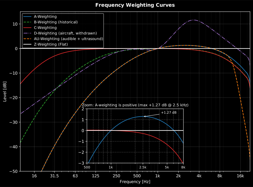## Weighting Curves (IEC 61672-1) The A-weighting transfer function: $$ R_\mathrm{A}(f) = \frac{12194^2 \cdot f^4}{(f^2 + 20.6^2)\sqrt{(f^2 + 107.7^2)(f^2 + 737.9^2)}(f^2 + 12194^2)} $$ $$ A(f) = 20 \log_{10}(R_\mathrm{A}(f)) + 2.00 $$ The digital filter is obtained from the analog poles/zeros via the bilinear transform. That transform compresses frequencies near Nyquist, so the default `high_accuracy` mode does not apply it to the printed prototype: it fits a prototype of the same structure whose response *at the warped frequencies* is the printed one's response at the true frequencies, and transforms that. See [Frequency Weighting](https://docs.jmrp.io/phonometry/signals/levels/weighting/). *The three IEC 61672-1 weighting curves realized by the library, with the small positive region of the A curve magnified. 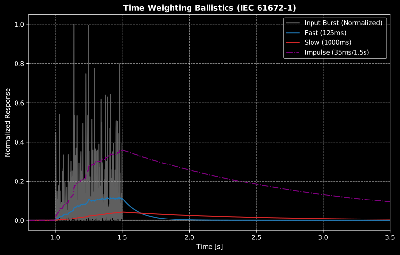The special B, D and AU curves are charted in [Special Weightings](https://docs.jmrp.io/phonometry/signals/levels/special-weightings/).* ## Time Integration Implemented as a first-order IIR exponential integrator: $$ y[n] = \alpha \cdot x^2[n] + (1 - \alpha) \cdot y[n-1] $$ $$ \alpha = 1 - \mathrm{e}^{-1 / (f_\mathrm{s} \cdot \tau)} $$ Where $\tau$ is the time constant (e.g., 125 ms for Fast). The default initial condition is $y[-1] = 0$. Use `initial_state='first'` to start from the first input energy, or pass a scalar/array with the previous mean-square output state. See [Why phonometry](https://docs.jmrp.io/phonometry/start/why-phonometry/) for the IEC 61672-1 tone-burst verification of this implementation. *The exponential integrator at the three standard time constants: Fast follows a burst, Slow smooths it and Impulse holds its peak.* ## G-weighting (ISO 7196) The G curve extends frequency weighting into the infrasound range. ISO 7196:1995 Table 1 (p. 2) defines it by four zeros at the origin and four complex-conjugate pole pairs, given as coordinates in Hz (multiplied by $2\pi$ to obtain rad/s): $$ z_{1..4} = 0, \qquad p = 2\pi \left\lbrace -0.707 \pm j0.707,\ -19.27 \pm j5.16,\ -14.11 \pm j14.11,\ -5.16 \pm j19.27 \right\rbrace \ \text{Hz} $$ The gain $k$ is chosen so that the response is exactly **0 dB at 10 Hz** (clause 4): $$ k = \left| \frac{\prod_i (j\omega_{10} - p_i)}{\prod_i (j\omega_{10} - z_i)} \right|, \qquad \omega_{10} = 2\pi \cdot 10 \ \text{rad/s} $$ The four zeros against eight poles shape the characteristic response: a rise of approximately **+12 dB/octave between 1 Hz and 20 Hz**, with roll-offs of approximately **24 dB/octave** below 1 Hz and above 20 Hz. Infrasound needs its own curve because near the hearing threshold the perceived loudness of very-low-frequency tones grows much more steeply with sound pressure level than at mid frequencies (a small dB increase above threshold produces a large loudness jump), so the A curve (anchored at 1 kHz) grossly misrepresents infrasonic annoyance. *The shape those four zeros and four pole pairs make, against the ISO 7196 Table 2 nominal values: 0 dB at the 10 Hz anchor, the +12 dB/octave climb through the infrasound decade below it, and the two 24 dB/octave roll-offs that fence the curve off below 1 Hz and above 20 Hz.* Since G acts on 0.25 Hz – 315 Hz, far below the Nyquist frequency at audio rates, the frequency warping of the plain bilinear transform (applied without prewarping) is negligible there: about 0.014 % at 315 Hz for $f_\mathrm{s} = 48$ kHz, under 0.01 dB on the response. The default design still fits the prototype at the sample rate as it does for A and C, which costs nothing here and matters at the low rates infrasound is often recorded at, where 315 Hz approaches Nyquist. See the [Special Weightings guide](https://docs.jmrp.io/phonometry/signals/levels/special-weightings/) for usage. ## Event and dose metrics **Sound exposure level** (SEL; $L_{\mathrm{A}E}$ with A-weighting, IEC 61672-1:2013) normalizes the energy of a discrete event (aircraft flyover, train pass) to a 1 s reference duration: $$ \mathrm{SEL} = L_{\mathrm{eq},T} + 10 \log_{10}\left(\frac{T}{T_0}\right), \qquad T_0 = 1\ \text{s} $$ *What the formula does to an event: the pass-by is replaced by a one-second block of the same total energy, which is why SEL exceeds the event's $L_\mathrm{eq}$ whenever the event lasts longer than a second, and why two events of the same SEL are interchangeable in a dose even when one is loud and short and the other quiet and long.* **Sound exposure** $E$ (IEC 61252, 3.1) is the time integral of the squared A-weighted sound pressure, expressed in pascal-squared hours: $$ E = \int_0^T p_\mathrm{A}^2(t)\ dt = \overline{p_\mathrm{A}^2} \cdot T \quad [\text{Pa}^2\text{h}] $$ When the recording is a representative sample of a longer shift, $E$ scales the measured mean square by the actual exposure duration. The **normalized 8 h level** (IEC 61252, 3.3) converts exposure to the steady level that carries the same energy over a nominal working day: $$ L_\mathrm{EX,8h} = 10 \log_{10}\left(\frac{E}{8\ \text{h} \cdot p_0^2}\right), \qquad p_0 = 20\ \mu\text{Pa} $$ It is identical to $L_\mathrm{EP,d}$ of Directive 86/188/EEC and $L_\mathrm{EX,8h}$ of ISO 1999 (IEC 61252, 3.3 NOTES 5–6). The anchor of IEC 61252 (3.3 NOTE 4): an exposure of **3.2 Pa²h corresponds to $L_\mathrm{EX,8h}$ of exactly 90 dB**. **$L_\mathrm{Cpeak}$** (IEC 61672-1:2013, subclause 5.13) is the absolute maximum of the C-weighted sound pressure expressed in dB, $L_\mathrm{Cpeak} = 20\log_{10}(\max|p_\mathrm{C}(t)|/p_0)$, the quantity behind the 135/137/140 dB(C) occupational action limits. The implementation is verified against the one-cycle and half-cycle reference responses of Table 5. See the [Levels guide](https://docs.jmrp.io/phonometry/signals/levels/levels/) for usage and the [Calibration guide](https://docs.jmrp.io/phonometry/signals/metrology/calibration/) for absolute-scale setup. ## Sound intensity (IEC 61043) Sound intensity is the time-averaged acoustic power flux $I = \overline{p u}$. 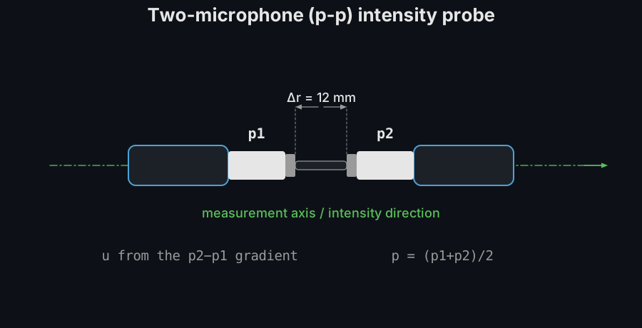The particle velocity follows from **Euler's equation** (linearized conservation of momentum): $$ \rho_0 \frac{\partial u}{\partial t} = -\frac{\partial p}{\partial r} $$ A p-p probe approximates the pressure gradient by the **finite difference** of two microphones a spacer distance $\Delta r$ apart (IEC 61043:1994, definition 3.2): $$ p = \frac{p_1 + p_2}{2}, \qquad u = -\frac{1}{\rho_0 \Delta r} \int (p_2 - p_1)\ dt, \qquad I = \overline{p\ u} $$ For stationary signals the same estimator has an exact frequency-domain form through the imaginary part of the one-sided **cross spectrum** $G_{12}$ of the two pressures; the implementation estimates it with Welch-averaged, Hann-windowed segments: $$ I(f) = -\ \frac{\mathrm{Im}\lbrace G_{12}(f)\rbrace}{2 \pi f\ \rho_0\ \Delta r} $$ The finite difference underestimates the true plane-wave intensity by the factor $$ \frac{\sin(k \Delta r)}{k \Delta r}, \qquad k = \frac{2 \pi f}{c} $$ IEC 61043 clause 7.3 specifies the probe intensity response with exactly this argument and Table 3 tabulates it (e.g. −10.5 dB at 6.3 kHz for a 25 mm spacer). Below $f = 0.1 c / \Delta r$ (i.e. $k \Delta r$ under 0.63) the bias stays within about 0.3 dB; `bias_correction` provides the reciprocal factor per band and `max_valid_frequency` the bound. 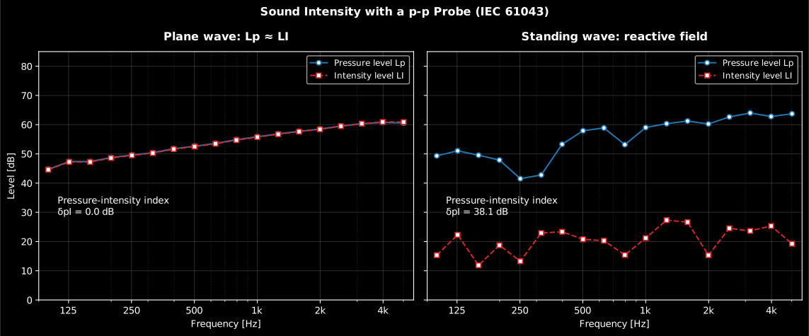The **pressure-intensity index** $\delta_{pI} = L_p - L_I$ measures how reactive the field is: in a free plane progressive wave it equals $10 \log_{10}(\rho_0 c / 400) = 0.14$ dB, while large values flag reactive or noisy fields in which the inter-channel phase error dominates. ISO 9614-1:1993 Annex A generalizes it over a measurement surface as the indicator F2 (with F3 for negative partial power and F4 for field non-uniformity), and the instrument's **dynamic capability** $L_\mathrm{d} = \delta_{pI0} - K$ (pressure-residual intensity index minus the bias error factor: 10 dB for grades 1/2, 7 dB for grade 3) must exceed F2 for the measurement to be valid (criterion 1). See the [Sound Intensity guide](https://docs.jmrp.io/phonometry/devices/emission/intensity/) for usage. *The p-p estimator in the two limiting fields: the gap between $L_p$ and $L_I$ is the pressure-intensity index that flags reactive fields.* ## Measurement uncertainty (ISO/IEC Guide 98-3: GUM and Supplement 1) Domain budgets like ISO 12999-1 and ISO 9612 Annex C are instances of the general framework of the GUM (ISO/IEC Guide 98-3:2008). Given a measurement model $y = f(x_1, \ldots, x_N)$, the law of propagation of uncertainty (clause 5) combines the input standard uncertainties through sensitivity coefficients: $$ u_\mathrm{c}^2(y) = \sum_{i=1}^{N} \left( \frac{\partial f}{\partial x_i} \right)^2 u^2(x_i), $$ generalized to $(c \odot u)^{\top} r\ (c \odot u)$ for correlated inputs. The sensitivities are obtained by central differences on the user's model callable (step scaled to $10^{-3}$ of each input uncertainty), so no hand-derived partials are needed. Type B inputs enter through the clause 4.3 half-width rules: rectangular $a/\sqrt{3}$ (4.3.7), triangular $a/\sqrt{6}$ (4.3.9), U-shaped $a/\sqrt{2}$. The expanded uncertainty $U = k\,u_\mathrm{c}$ takes $k$ from the t-distribution at the Welch–Satterthwaite effective degrees of freedom (Annex G.4): $$ \nu_{\mathrm{eff}} = \frac{u_\mathrm{c}^4}{\sum_i u_i^4 / \nu_i}. $$ **Supplement 1** (ISO/IEC Guide 98-3-1:2008) propagates the full distributions instead: $10^6$ Monte Carlo draws (clause 6.4) through the same model give $u(y)$ and the probabilistically symmetric coverage interval from the $\frac{1}{2}(1 \mp p)$ fractiles (clause 7.7): the route when the model is non-linear or the output visibly non-Gaussian. The Guides' own examples are reproduced: the four-term additive model gives $u_\mathrm{c} = 2.0$ and the Monte Carlo 95 % interval $\pm 3.88$ of Supplement 1 clause 9.2/Table 3 (four rectangular inputs; the output is nearly trapezoidal, not Gaussian, so the interval is narrower than $\pm 1.96\,u$), and the GUM Annex H.1 end-gauge example gives $k = t_{0.99}(\nu_{\mathrm{eff}} = 16) = 2.92$ and $U_{99} = 93$ nm. *The two routes on one problem, an A-weighted level, not the Supplement 1 four-term example quoted above. Left is the law of propagation as a budget: one bar per input, so the term worth reducing is visible. Right is the Supplement 1 route: the Monte Carlo output distribution with the GUM Gaussian drawn over it and the 95 % coverage interval shaded. Here the two agree, which is what clause 8 calls validation; where the model is non-linear or the output visibly non-Gaussian the histogram departs from the curve and the interval is read off the fractiles instead.* See the [GUM Uncertainty guide](https://docs.jmrp.io/phonometry/signals/metrology/gum-uncertainty/) for usage. ## References - Oppenheim, A. V., & Schafer, R. W. (2010). *Discrete-time signal processing* (3rd ed.). Pearson. ISBN 978-0-13-198842-2. [Open Library record](https://openlibrary.org/isbn/9780131988422). The digital-filter theory behind the SOS cascades, the bilinear transform and the multirate decimation of the filter-bank design section. - Smith, J. O. *Introduction to digital filters with audio applications* (online book). Center for Computer Research in Music and Acoustics (CCRMA), Stanford University. [ccrma.stanford.edu/~jos/filters](https://ccrma.stanford.edu/~jos/filters/). Free companion treatment of the classical filter prototypes and their magnitude responses. - Fahy, F. J. (1995). *Sound intensity* (2nd ed.). E&FN Spon. ISBN 978-0-419-19810-9. [doi:10.4324/9780203475386](https://doi.org/10.4324/9780203475386). The physics of the p-p estimator: active intensity, the finite-difference bias and the phase-mismatch error budget. - International Electrotechnical Commission. (2014). *Electroacoustics — Octave-band and fractional-octave-band filters — Part 1: Specifications* (IEC 61260-1:2014). [IEC webstore](https://webstore.iec.ch/en/publication/5063). The base-10 mid-band and band-edge definitions of the octave-band section and the class masks the banks are verified against. - International Electrotechnical Commission. (2013). *Electroacoustics — Sound level meters — Part 1: Specifications* (IEC 61672-1:2013). [IEC webstore](https://webstore.iec.ch/en/publication/5708). The A/C/Z weighting curves, the exponential time integration and the SEL and LCpeak definitions of the event-metric section. - International Electrotechnical Commission. (1993). *Electroacoustics — Instruments for the measurement of sound intensity — Measurements with pairs of pressure sensing microphones* (IEC 61043:1993; adopted in Europe as EN 61043:1994). [IEC webstore](https://webstore.iec.ch/en/publication/4353). The p-p instrument standard: the cross-spectral estimator and the pressure-residual intensity index behind the dynamic capability. - International Organization for Standardization. (1993). *Acoustics — Determination of sound power levels of noise sources using sound intensity — Part 1: Measurement at discrete points* (ISO 9614-1:1993). [iso.org catalogue](https://www.iso.org/standard/17427.html). The surface indicators F2–F4 that generalize the pressure-intensity index over a measurement surface. - Joint Committee for Guides in Metrology. (2008). *Evaluation of measurement data — Guide to the expression of uncertainty in measurement* (JCGM 100:2008, the GUM). BIPM. [doi:10.59161/JCGM100-2008E](https://doi.org/10.59161/JCGM100-2008E), [free PDF](https://www.bipm.org/documents/20126/2071204/JCGM_100_2008_E.pdf). The law of propagation of uncertainty and the Welch–Satterthwaite expanded uncertainty of the GUM section. - Joint Committee for Guides in Metrology. (2008). *Evaluation of measurement data — Supplement 1 to the "Guide to the expression of uncertainty in measurement" — Propagation of distributions using a Monte Carlo method* (JCGM 101:2008). BIPM. [doi:10.59161/JCGM101-2008](https://doi.org/10.59161/JCGM101-2008), [free PDF](https://www.bipm.org/documents/20126/2071204/JCGM_101_2008_E.pdf). The Monte Carlo propagation of distributions and its coverage-interval construction.