Source: https://docs.jmrp.io/phonometry/reference/theory/perception/ # Theory: Perception and Hearing This page collects the theory behind hearing and psychoacoustics: the equal-loudness contours, the Zwicker, Moore-Glasberg and Sottek loudness models, the sound-quality metrics tonality, roughness and sharpness, tone prominence, the speech metrics STI and SII, and the statistics of hearing thresholds and hearing loss. It is part of the [theory reference](https://docs.jmrp.io/phonometry/reference/theory/). 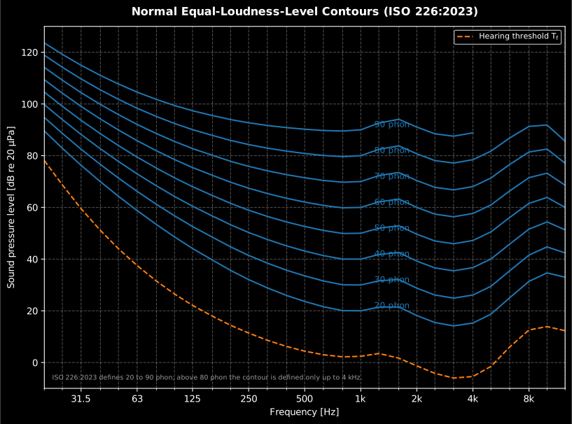## Equal-loudness contours (ISO 226:2023) A tone has a *loudness level* of $L_\mathrm{N}$ phon when it is judged equally loud as a 1 kHz pure tone at $L_\mathrm{N}$ dB SPL. ISO 226:2023 Formula (1) (clause 4.1, p. 2) gives the SPL of a pure tone at frequency $f$ that reaches loudness level $L_\mathrm{N}$: $$ L_f = \frac{10}{\alpha_f} \log_{10}\left[ \left(4 \cdot 10^{-10}\right)^{0.3 - \alpha_f} \left( 10^{\ 0.03 L_\mathrm{N}} - 10^{\ 0.072} \right) + 10^{\ \alpha_f (T_f + L_\mathrm{U})/10} \right] - L_\mathrm{U} $$ Formula (2) (clause 4.2) inverts it, returning the loudness level of a tone at SPL $L_f$: $$ L_\mathrm{N} = \frac{100}{3} \log_{10}\left[ \frac{10^{\ \alpha_f (L_f + L_\mathrm{U})/10} - 10^{\ \alpha_f (T_f + L_\mathrm{U})/10}}{\left(4 \cdot 10^{-10}\right)^{0.3 - \alpha_f}} + 10^{\ 0.072} \right] $$ The three parameters come from Table 1 (p. 4), tabulated at the 29 preferred third-octave frequencies of ISO 266 from 20 Hz to 12.5 kHz: - $\alpha_f$: exponent for loudness perception at frequency $f$, - $L_\mathrm{U}$: magnitude of the linear transfer function, normalized at 1 kHz ($L_\mathrm{U} = 0$ at 1 kHz), - $T_f$: threshold of hearing at $f$, in dB. The standard specifies **no interpolation** between the tabulated frequencies. Formula (1) is specified for **20 phon to 90 phon** between 20 Hz and 4 kHz, and only up to **80 phon between 5 kHz and 12.5 kHz**; above 80 phon the contour therefore stops at 4 kHz. Values outside these limits from Formula (2) are extrapolations the standard labels as informative only. *The ISO 226:2023 contours from Formula (1), 20 to 90 phon, with the hearing threshold.* See the [Loudness guide](https://docs.jmrp.io/phonometry/perception/psychoacoustics/loudness/) for usage. ## Tone prominence: TNR and PR (ECMA-418-1) Both methods operate on a Hann-windowed, RMS-averaged power spectrum (clauses 11.1 / 12.1) and use the clause 10 critical-band model. The critical bandwidth centred on a tone at $f$ is (Formula 2): $$ \Delta f_\mathrm{c} = 25.0 + 75.0 \left(1.0 + 1.4 \left(\tfrac{f}{1000}\right)^2\right)^{0.69} \ \text{Hz} $$ Band edges are placed **arithmetically** for $f \le 500$ Hz (Formulae 4–5): $f_{1,2} = f \mp \Delta f_\mathrm{c} / 2$, and **geometrically** above (Formulae 7–8): $f_1 = -\Delta f_\mathrm{c}/2 + \sqrt{\Delta f_\mathrm{c}^2 + 4 f^2}/2$, $f_2 = f_1 + \Delta f_\mathrm{c}$. **TNR** (clause 11). The tone band spans the spectral minima on both sides of the peak within 15 % of $\Delta f_\mathrm{c}$ (clause 11.2). The tone power subtracts the straight line connecting the band-edge bins (Formula 9): over $N$ tone-band bins, $P_t = \sum_k P_k - (P_{\text{lo}} + P_{\text{hi}})\ N/2$. The masking-noise power is the remaining critical-band power rescaled to the full critical bandwidth (Formula 10): $P_n = (P_{\text{band}} - P_t) \cdot \Delta f_\mathrm{c} / \Delta f_{\text{band}}$, and $\mathrm{TNR} = 10\log_{10}(P_t/P_n)$ (Formula 11). The prominence criterion (Formulae 12–13) is $$ \mathrm{TNR}_{\text{crit}} = \begin{cases} 8.0 + 8.33 \log_{10}(1000/f_\mathrm{t}) \ \text{dB} & f_\mathrm{t} < 1\ \text{kHz} \\ 8.0 \ \text{dB} & f_\mathrm{t} \ge 1\ \text{kHz} \end{cases} $$ **PR** (clause 12) compares the level of the critical band centred on the tone, $L_\mathrm{M}$, with the mean power of the two **contiguous** critical bands $L_\mathrm{L}$, $L_\mathrm{U}$ (edges from the fitted Formulae 21–22 with Tables 2–3): $\mathrm{PR} = 10\log_{10} P_\mathrm{M} - 10\log_{10}\left[(P_\mathrm{L} + P_\mathrm{U})/2\right]$ (Formula 23). For $f_\mathrm{t} \le 171.4$ Hz the lower band is truncated at 20 Hz and its power rescaled to a **100 Hz bandwidth** (Formula 24). The criterion (Formulae 25–26) is 9.0 dB at $f_\mathrm{t} \ge 1$ kHz, rising as $9.0 + 10.0\log_{10}(1000/f_\mathrm{t})$ below. Tones are assessed within the 89.1 Hz – 11.2 kHz range of interest (clauses 11.5 / 12.6). *The TNR criterion drawn rather than evaluated, over the 89.1 Hz – 11.2 kHz range of interest, with one assessed tone on it. Because the criterion is $8.0 + 8.33\log_{10}(1000/f_\mathrm{t})$ below 1 kHz and flat above, the same tone-to-noise ratio is judged against a different threshold at every frequency: the example tone clears its 13.0 dB threshold at 250 Hz by 2.1 dB, while a 10 dB tone would be prominent anywhere above 1 kHz and not prominent here.* See the [Prominent Discrete Tones guide](https://docs.jmrp.io/phonometry/perception/psychoacoustics/tone-prominence/) for usage. 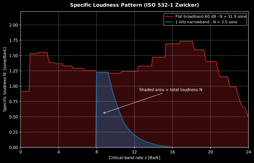## Zwicker loudness (ISO 532-1) The ear analyzes sound in **critical bands**: frequency regions within which energy is summed before loudness is formed. The **Bark scale** maps frequency to critical-band rate $z$, 0 to 24 Bark, and ISO 532-1:2017 samples the specific loudness $N'(z)$ at 0.1-Bark steps (240 values). The implementation is a clean-room port of the standard's normative reference program (Annex A.4) and proceeds in stages: 1. **One-third-octave levels**: 28 bands, 25 Hz to 12.5 kHz (the Annex A filterbank at 48 kHz, Tables A.1/A.2). For time-varying sounds the squared band outputs are smoothed by three cascaded low-passes with $\tau = 2/(3 f_\mathrm{c})$ ($f_\mathrm{c}$ capped at 1 kHz) and sampled every 2 ms. 2. **Low-frequency grouping**: the 11 bands up to 250 Hz receive the equal-loudness corrections of Table A.3 and are summed into the first three critical bands (25–80, 100–160, 200–250 Hz). 3. **a0 transmission**: the outer/middle-ear transfer correction of Table A.4 (plus the diffuse-field difference of Table A.5 when `field='diffuse'`) yields the critical-band levels $L_E$. 4. **Core loudness**: each of the 20 critical bands is transformed with the threshold-in-quiet levels $L_\mathrm{TQ}$ of Table A.6 (after the bandwidth adaptation DCB of Table A.7): $$ N_c = \max\left(0,\ 0.0635 \cdot 10^{0.025 L_\mathrm{TQ}} \left[ \left( 1 - s + s \cdot 10^{(L_E - L_\mathrm{TQ})/10} \right)^{0.25} - 1 \right]\right) \ \text{sone/Bark}, \qquad s = 0.25 $$ (the reference program's form of Zwicker's loudness transformation; bands below threshold contribute zero). 5. **Slopes**: level-dependent upper masking slopes (steepness per specific-loudness range and critical band, Tables A.8/A.9) attach decaying flanks toward higher $z$; the total loudness is the area under the pattern: $$ N = \int_0^{24} N'(z)\ dz \ \ \text{sone} $$ For time-varying sounds a nonlinear temporal decay (time constants 5/15/75 ms, clause 6.3) and the duration-dependent weighting of the total loudness (3.5 ms and 70 ms low-passes weighted 0.47/0.53, also clause 6.3) precede the 500 Hz loudness-vs-time output (clause 6.3) and the percentile values N5/N10 (clause 6.4). **Sone and phon** are tied together by the 1 kHz anchor (1 sone = 40 phon; clause 5.6): $$ N = 2^{(L_\mathrm{N} - 40)/10} \ \text{sone} \qquad \Longleftrightarrow \qquad L_\mathrm{N} = 40 + 10 \log_2 N \ \text{phon} \qquad (N \ge 1) $$ below 1 sone the reference program uses $L_\mathrm{N} = 40 (N + 0.0005)^{0.35}$, floored at 3 phon. *Specific loudness N′(z) over the Bark axis: energy spread over many critical bands sums to more sones than the same band level in a single band.* See the [Loudness guide](https://docs.jmrp.io/phonometry/perception/psychoacoustics/loudness/) for usage. ## Advanced loudness models & sound quality ISO 532-1 is one of three loudness models; two newer families refine the auditory front-end and add the sound-quality metrics tonality and roughness. ### Moore-Glasberg loudness (ISO 532-2:2017, ISO 532-3:2023) Instead of Zwicker's fixed critical bands, the Moore-Glasberg model forms a continuous **excitation pattern** on the ERB-number ("Cam") scale using level-dependent **rounded-exponential (roex)** auditory filters. As a function of the normalized frequency deviation $g = |f - f_\mathrm{c}| / f_\mathrm{c}$ from a filter centred at $f_\mathrm{c}$, the filter weighting is $$ W(g) = (1 + p\ g)\ \mathrm{e}^{-p\ g} $$ where the slope $p$ grows with the source level, broadening the lower skirt as level rises (ISO 532-2, Formulae 2–5); this reproduces the upward spread of masking. Passing the stimulus intensity through every filter gives the excitation $E(i)$, and a compressive law maps it to the **specific loudness** $N'(i)$ in sone/Cam (Formulae 7–9), of the mid-level form $$ N'(i) = C \left[ \left( G\ \frac{E(i)}{E_0} + A \right)^{\alpha} - A^{\alpha} \right] $$ with the calibration constant $C = 0.0617$ sone/Cam (ISO 532-2; $0.063$ in ISO 532-3). The total loudness is the area under the pattern, $$ N = \int N'(i)\ di \ \ \text{sone} $$ and a binaural-inhibition stage (Formulae 10–13) combines the ears so a diotic sound is louder than the same sound at one ear. The 1 kHz / 40 dB SPL anchor gives exactly 1 sone. **ISO 532-3** makes this time-varying. A running spectrum from six parallel Hann-windowed FFTs (segment lengths 2–64 ms, each contributing its own frequency range, updated every $T_0 = 1$ ms) drives the same excitation and specific-loudness chain, integrated by two cascaded first-order smoothers with $\alpha = 1 - \mathrm{e}^{-T_0 / \tau}$, $$ S(t) = \alpha\ x(t) + (1 - \alpha)\ S(t - 1) $$ using a fast time constant on the attack and a slower one on the release. This yields the **short-term loudness** $S'(t)$ (attack/release near 20–30 ms) and the **long-term loudness** $S''(t)$ (near 0.1–0.75 s); the peak long-term loudness $N_{\max} = \max_t S''(t)$ predicts the loudness of sounds up to about 5 s. ### Sottek Hearing Model (ECMA-418-2:2025) ECMA-418-2 builds all three of its metrics on one auditory front-end (Clause 5): an outer/middle-ear filter, a bank of 53 overlapping gammatone-like band-pass filters spaced on the Bark_HMS scale ($z = 0.5$ to $26.5$), half-wave rectification, and a short-block RMS $\tilde{p}(l, z)$ per band $z$ and time block $l$. A compressive nonlinearity (Formula 23) turns the band RMS into the **specific basis loudness** $N'_{\mathrm{basis}}(l, z)$, whose calibration constant $c_\mathrm{N}$ fixes a 1 kHz / 40 dB SPL tone at 1 sone_HMS. The loudness assembles the tonal and noise loudness (below) over bands and time (Formulae 113–117); it grows about $1.65\times$ per 10 dB, more slowly than Zwicker's factor of 2, an intrinsic property of the Sottek summation. *The divergence stated above, drawn on the one signal all three models are calibrated on. They pass together through about 1 sone at 40 dB (the Sottek front end returns 0.9845 sone$_\mathrm{HMS}$ there) and then separate: Zwicker's curve doubles every 10 dB, the Sottek curve rises by about 1.65× over the same step. That is a difference between auditory summations, not a calibration error, and it is why a sone value without its model attached cannot be compared with anything.* ### Tonality: autocorrelation of the band signal (ECMA-418-2) A tonal component is periodic, so it survives in the **autocorrelation function** (ACF) of a band's rectified signal while broadband noise decorrelates. For each band the unbiased ACF of the block is $$ \phi_z(m) = \frac{1}{M - m} \sum_{n=0}^{M - 1 - m} p_z(n)\ p_z(n + m) $$ A windowed spectral estimate of $\phi_z$ separates a **tonal loudness** $N'_{\mathrm{tonal}}(l, z)$ from the **noise loudness** $N'_{\mathrm{noise}}(l, z)$ (Formulae 36–48). The specific tonality is the tonal loudness scaled by a smooth signal-to-noise gate $q(l)$ (Formulae 49–51), $$ T'(l, z) = c_\mathrm{T}\ q(l)\ N'_{\mathrm{tonal}}(l, z) $$ and the single value $T$ (tu_HMS) is the gated time-average of the per-block maximum over bands (Formulae 61–64). The constant $c_\mathrm{T}$ fixes the 1 kHz / 40 dB tone at 1 tu_HMS, and the band of the ACF peak gives the tonal frequency $f_{\mathrm{ton}}$. ### Roughness: envelope modulation (ECMA-418-2) Roughness is the sensation of fast (roughly 20–300 Hz) amplitude modulation, strongest near 70 Hz. From each band's envelope $p_\mathrm{E}(n)$ (Hilbert magnitude), a modulation spectrum is formed and weighted by a modulation-rate function peaking near 70 Hz and by the modulation depth; correlating the modulation across neighbouring bands and applying the specified temporal filtering yields the **specific roughness** $R'(l_{50}, z)$ and the time-dependent roughness $$ R(l_{50}) = \sum_z R'(l_{50}, z) \ \ \text{asper} $$ (Formulae 65–111). The single value $R$ is the 90th percentile of $R(l_{50})$ over time (Clause 7.1.10); the constant $c_\mathrm{R}$ (Formula 104) calibrates the reference sound (a 1 kHz carrier 100 % amplitude-modulated at 70 Hz at 60 dB SPL) to 1 asper. *The modulation-rate weighting the formulae above apply, and the reason the range "roughly 20–300 Hz, strongest near 70 Hz" is a band-pass and not a threshold: the same 1 kHz carrier modulated slowly is heard as fluctuation strength, peaking near 4–6 Hz, and modulated fast is heard as roughness, peaking near 70 Hz. Between the two peaks the sensation changes name, not degree.* ### Sharpness (DIN 45692) Sharpness condenses the high-frequency emphasis of a sound into one number: the $g(z)$-weighted first moment of the ISO 532-1 stationary specific-loudness pattern (DIN 45692:2009-08, Equation 1): $$ S = k\ \frac{\int_0^{24} N'(z)\ g(z)\ z\ dz}{\int_0^{24} N'(z)\ dz} \ \text{acum}, \qquad g(z) = \begin{cases} 1 & z \le 15.8\ \text{Bark} \\ 0.15\ \mathrm{e}^{0.42 (z - 15.8)} + 0.85 & z > 15.8\ \text{Bark} \end{cases} $$ evaluated on the same 240-bin, 0.1-Bark grid. The constant $k$ is not hard-coded but derived from the calibration requirement (clause 6): a critical-band-wide narrowband noise 920–1080 Hz at 60 dB SPL scores exactly 1 acum, and the derived $k = 0.108$ lands inside the normative window $0.105 \le k < 0.115$ (clause 5.2). The informative Annex B weightings are provided under the same 1-acum anchor: von Bismarck (knee at 15 Bark, $0.2\ \mathrm{e}^{0.308(z-15)} + 0.8$) and Aures (loudness-dependent, $g(z) = 0.078\ (\mathrm{e}^{0.171 z}/z)\ N/\ln(0.05 N + 1)$). The Table A.2 narrow-band targets are reproduced within the clause 6 tolerance (5 % or 0.05 acum): 0.38 acum at 250 Hz, 1.00 at 1 kHz, 1.78 at 2.5 kHz, 2.82 at 4 kHz. *The three $g(z)$ weightings of the formula above on one axis: DIN with its 15.8 Bark knee, von Bismarck with its 15 Bark knee, and the loudness-dependent Aures curve, which is why the choice of weighting changes a sharpness value only for sounds with energy above the knee (15 to 15.8 Bark, about 2.5 to 3 kHz) and leaves everything below it untouched.* See the [Sound Quality Metrics guide](https://docs.jmrp.io/phonometry/perception/psychoacoustics/sound-quality/) for usage. ## Modulation transfer and STI (IEC 60268-16) Speech intelligibility rides on the slow intensity modulations of the speech envelope. The **modulation transfer function** $m(F)$ of a transmission channel is the ratio of received to emitted modulation depth of the octave-band intensity envelope at modulation frequency $F$; the full STI evaluates it at the 14 one-third-octave modulation frequencies 0.63–12.5 Hz in the seven octave bands 125 Hz – 8 kHz (A.2.2). From a measured impulse response the **Schroeder closed form** gives it directly (indirect method): $$ m_k(f_m) = \frac{\left| \int_0^{\infty} h_k^2(t)\ \mathrm{e}^{-j 2 \pi f_m t}\ dt \right|}{\int_0^{\infty} h_k^2(t)\ dt} $$ Steady background noise multiplies each band's $m$ by the intensity ratio (the noise term): $$ m'_k = m_k \cdot \frac{I_k}{I_k + I_{\mathrm{n},k}} = \frac{m_k}{1 + 10^{-\mathrm{SNR}_k/10}} $$ and when absolute band levels are known the full correction $m'_k = m_k I_k / (I_k + I_{\mathrm{am},k} + I_{\mathrm{rt},k} + I_{\mathrm{n},k})$ adds the auditory masking intensity $I_{\mathrm{am},k}$ (from the next lower octave band, Table A.2) and the absolute reception threshold $I_{\mathrm{rt},k}$ (Table A.3). Each corrected $m$ maps to an **effective SNR**, clipped to the ±15 dB range where intelligibility actually varies, then to a transmission index (A.5.4/A.5.5): $$ \mathrm{SNR}_{\mathrm{eff}} = 10 \log_{10} \frac{m}{1 - m}\ \text{dB}, \qquad \mathrm{TI} = \frac{\mathrm{SNR}_{\mathrm{eff}} + 15}{30} $$ The band MTI is the mean TI over the modulation frequencies, and the STI weights the bands with the male factors $\alpha_k$, $\beta_k$ of Ed. 5 Table A.1 (A.5.6): $$ \mathrm{STI} = \sum_{k=1}^{7} \alpha_k\ \mathrm{MTI}_k - \sum_{k=1}^{6} \beta_k \sqrt{\mathrm{MTI}_k\ \mathrm{MTI}_{k+1}} $$ truncated to 1.0. STIPA (Annex B) samples the same physics with just two modulation frequencies per band (Table B.1) on a test signal with source modulation index 0.55; the received depths are measured by sine/cosine correlation of the ~100 Hz low-passed intensity envelopes $I_k(t)$ over an integer number of modulation periods: $$ m_{dr} = \frac{2 \sqrt{\left( \sum_t I_k(t) \sin 2 \pi f_m t \right)^2 + \left( \sum_t I_k(t) \cos 2 \pi f_m t \right)^2}}{\sum_t I_k(t)}, \qquad m = \frac{m_{dr}}{0.55} $$ *The seven $\mathrm{MTI}_k$ the weighted sum above consumes, for a hall with $T = 0.9$ s and a 15 dB speech-to-noise ratio. Each bar is already the mean of 14 transmission indices, so this is two stages of averaging below the raw $m(F)$; the bars sit within 0.06 of one another, which is the case in which the $\beta_k$ redundancy terms subtract almost nothing and the STI is close to the plain $\alpha$-weighted mean.* *The end of the chain rather than its middle: what the Schroeder closed form does to the STI as reverberation grows, against the Annex F rating bands. The curve falls steeply through the range where a room is still usable and flattens once the modulation has already been destroyed, which is why halving a long reverberation time buys less intelligibility than halving a short one.* See the [Speech Transmission Index guide](https://docs.jmrp.io/phonometry/perception/speech/speech-transmission/) for usage. ## Speech Intelligibility Index (ANSI S3.5) Where the STI characterizes a transmission channel, the SII (ANSI S3.5-1997) predicts intelligibility from what the listener can actually hear: 18 one-third-octave bands 160 Hz – 8 kHz, each contributing its band importance $I_i$ (Table 3, $\sum I_i = 1$, peaking near 2 kHz). All inputs are equivalent spectrum levels (clauses 3.11/3.55). Speech masks itself upward: each band's masking spectrum $Z_i$ (clause 5.4) accumulates the lower bands along slopes $C_i = -80 + 0.6\,(B_i + 10 \log_{10} f_i - 6.353)$ dB, and the disturbance is the **larger** of masking and hearing floor, $D_i = \max(Z_i, X'_i)$ (clause 5.6), with $X'_i = X_i + T'_i$ the reference internal noise spectrum plus the listener's hearing-threshold shift (clauses 5.5/5.6). The band audibility clips the speech-to-disturbance margin into $[0, 1]$ (clause 5.8), a level-distortion factor discounts overly loud presentation (clause 5.7), and the index sums (clause 6): *The importance function is where the speech cues are, and all four band procedures below agree about it: the same rise to a maximum near 2 kHz, the same total of 1.0 redistributed over wider or narrower bands, which is why the octave steps stand at 0.265 where the one-third-octave steps stand at 0.090. A band lost at 2 kHz costs several times what the same band costs at 160 Hz.* $$ A_i = \operatorname{clip}\Big( \frac{E'_i - D_i + 15}{30},\ 0,\ 1 \Big), \qquad L_i = \operatorname{clip}\Big( 1 - \frac{E'_i - U_i - 10}{160},\ 0,\ 1 \Big), \qquad \mathrm{SII} = \sum_{i=1}^{18} I_i\ L_i\ A_i . $$ The same chain runs over the standard's other three band tables, selected with `method=`: the 21 critical bands of Table 1, the 17 equally-contributing critical bands of Table 2 and the 6 octave bands of Table 4. Those three express the masking slope through the tabulated band width, $C_i = -80 + 0.6\,(B_i + 10 \log_{10} W_i)$, which is the same formula the $10 \log_{10} f_i - 6.353$ above abbreviates for a one-third-octave band; the octave-band procedure omits the spread of masking altogether, since an octave band is already wider than the spread being modelled. The Table 3 standard speech spectra for the normal, raised, loud and shout vocal efforts are built in (25.01 / 33.86 / 42.16 / 51.31 dB at 1 kHz); $U_i$ in the level-distortion factor is always the normal-effort spectrum. The anchor values: the normal-effort spectrum in quiet with normal hearing scores SII ≈ 0.996, the masking-spectrum reference values are matched to $10^{-4}$, and the vocal-effort spectra are cross-verified against the Google and CRAN reference implementations. *The four vocal efforts, in spectrum level rather than band level, which is why the normal-effort curve passes through 25.01 dB at 1 kHz rather than through the 60-odd dB a talker measures as a band level at a metre. Raising the effort does not lift the family uniformly: shouting adds 27.6 dB at 2.5 kHz, 26.3 dB at 1 kHz and **−1.6 dB** at 160 Hz, so the spectrum tilts as well as rises, and the extra effort is spent where the importance function above is largest.* See the [Speech Intelligibility guide](https://docs.jmrp.io/phonometry/perception/speech/speech-intelligibility/) for usage. 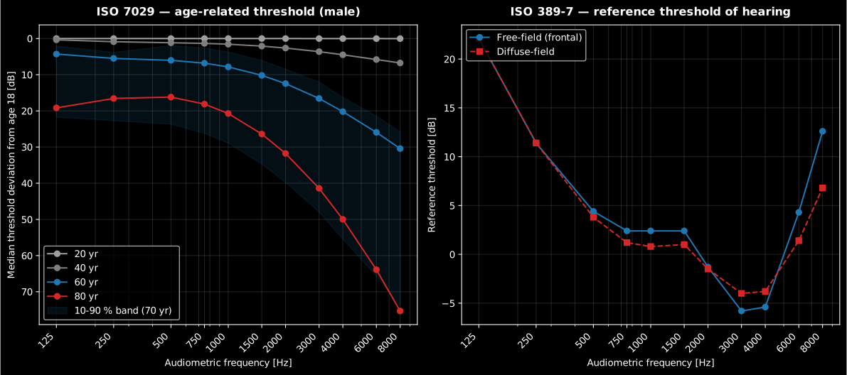## Hearing thresholds and presbycusis (ISO 389-7, ISO 7029) ISO 389-7:2005 Table 1 fixes the reference threshold of hearing of otologically normal young adults: the free-field and diffuse-field SPL corresponding to 0 dB HL at the 11 audiometric frequencies 125 Hz – 8 kHz (22.1 dB at 125 Hz for both fields, 2.4/0.8 dB free/diffuse at 1 kHz, diverging at high frequency to 12.6 vs 6.8 dB at 8 kHz). ISO 7029:2017 describes how that threshold shifts statistically with age: the median deviation from age 18 is (clause 4.2, Table 1) $$ \Delta H_\mathrm{md} = a\ (Y - 18)^b \ \text{dB}, $$ and any fractile follows a two-sided Gaussian model (clause 4.4), $\Delta H_Q = \Delta H_\mathrm{md} + z(Q)\ s$, using the upper spread $s_\mathrm{u}$ for $z \ge 0$ (worse than median) and the lower spread $s_\mathrm{l}$ otherwise, each a degree-5 polynomial in $Y - 18$ per sex and frequency (clause 4.3, Tables 2–5). At age 18 every deviation is zero by construction. The formulae are established to 80 years at and below 2 kHz and to 70 years above; beyond that the evaluation is an extrapolation. Anchors: at 60 years the medians evaluate to 7.85 dB (male, 1 kHz), 20.21 dB (male, 4 kHz) and 15.32 dB (female, 4 kHz), matching the Table 1 formula to $10^{-3}$. *The ISO 7029 median age shift with its fractile band (left) and the ISO 389-7 free- and diffuse-field reference thresholds (right).* See the [Hearing Threshold guide](https://docs.jmrp.io/phonometry/perception/hearing/hearing-threshold/) for usage. ## Noise-induced hearing loss (ISO 1999) ISO 1999:2013 predicts the permanent threshold shift a noise-exposed population accrues. The median noise-induced shift (NIPTS) for 10–40 years of exposure is (clause 6.3.1, Formula 2, Table 1): $$ N_{50} = \big[ u + v \log_{10}(t/t_0) \big]\ (L_\mathrm{EX,8h} - L_0)^2, \qquad t_0 = 1\ \text{yr}, $$ quadratic in the excess over the frequency-dependent onset level $L_0$ (75 dB at 4 kHz, the most sensitive band, up to 93 dB at 500 Hz) and zero below it; under 10 years it scales as $\log_{10}(t+1)/\log_{10} 11$ (Formula 3). Fractiles add the spread, $N_Q = N_{50} + z\ d_{u,l}$ with $d = (X + Y \log_{10} t)(L_\mathrm{EX,8h} - L_0)^2$ (clause 6.3.2, Formulae 4–7, Tables 2/3), clamped at zero. The library's `fractile` counts the fraction of the population with the *smaller* shift, so `fractile=0.9` is the most-susceptible decile (reliable range 0.05–0.95); ISO 1999's own $Q$ runs the other way, counting the percentage with worse hearing, so the same decile is $Q = 10\ \%$ there and in the Annex D column headings. The hearing threshold level associated with age and noise (HTLAN) combines NIPTS with the ISO 7029 age component at the same fractile through the compressed sum (clause 6.1, Formula 1): $$ H' = H + N - \frac{H\ N}{120}. $$ The Annex D worked examples (Tables D.1–D.4; e.g. 100 dB / 40 yr at 3 kHz: 29/38/60 dB at the 0.10/0.50/0.90 fractiles) are reproduced exactly at the standard's integer rounding, and the Formula 2 hand value at 4 kHz / 20 yr / 90 dB is $N_{50} = 12.94$ dB. *The model as an audiogram: 40 years at an 8 h-normalised 95 dB(A). The notch at 4 kHz is what makes noise-induced loss recognisable in a clinic, and it is here only because $L_0$ is lowest (75 dB) in that band. Mind the fractile direction the paragraph above states: the edge of the shaded band showing the **deeper** shift is the library's `fractile=0.90`, the most susceptible tenth, which ISO 1999 and its Annex D column headings label $Q = 10\ \%$. At 4 kHz this case runs 19.5 / 26.0 / 36.0 dB at `fractile` 0.10 / 0.50 / 0.90.* See the [Noise-Induced Hearing Loss guide](https://docs.jmrp.io/phonometry/perception/hearing/noise-induced-hearing-loss/) for usage. ## References - Fletcher, H., & Munson, W. A. (1933). Loudness, its definition, measurement and calculation. *The Journal of the Acoustical Society of America*, 5(2), 82-108. [doi:10.1121/1.1915637](https://doi.org/10.1121/1.1915637). The original equal-loudness measurements behind the contour concept of the first section. - Fastl, H., & Zwicker, E. (2007). *Psychoacoustics: Facts and models* (3rd ed.). Springer. [doi:10.1007/978-3-540-68888-4](https://doi.org/10.1007/978-3-540-68888-4). The critical-band, masking and loudness psychoacoustics underneath the Zwicker model and the sharpness and roughness sensations. - Houtgast, T., & Steeneken, H. J. M. (1985). A review of the MTF concept in room acoustics and its use for estimating speech intelligibility in auditoria. *The Journal of the Acoustical Society of America*, 77(3), 1069-1077. [doi:10.1121/1.392224](https://doi.org/10.1121/1.392224). The modulation-transfer framework of the STI section. - French, N. R., & Steinberg, J. C. (1947). Factors governing the intelligibility of speech sounds. *The Journal of the Acoustical Society of America*, 19(1), 90-119. [doi:10.1121/1.1916407](https://doi.org/10.1121/1.1916407). The articulation-band experiments behind the SII band-importance function. - Passchier-Vermeer, W. (1974). Hearing loss due to continuous exposure to steady-state broad-band noise. *The Journal of the Acoustical Society of America*, 56(5), 1585–1593. [doi:10.1121/1.1903482](https://doi.org/10.1121/1.1903482). A field study of the exposure-response relations later codified in ISO 1999. - International Organization for Standardization. (2023). *Acoustics — Normal equal-loudness-level contours* (ISO 226:2023). [iso.org catalogue](https://www.iso.org/standard/83117.html). The Formula (1)/(2) contour model and the Table 1 parameters of the equal-loudness section. - Ecma International. (2024). *ECMA-418-1: Psychoacoustic metrics for ITT equipment — Part 1: Prominent discrete tones* (3rd ed.). [Free PDF](https://ecma-international.org/wp-content/uploads/ECMA-418-1_3rd_edition_december_2024.pdf). The critical-band model and the TNR and PR procedures of the tone-prominence section. - International Organization for Standardization. (2005). *Acoustics — Reference zero for the calibration of audiometric equipment — Part 7: Reference threshold of hearing under free-field and diffuse-field listening conditions* (ISO 389-7:2005). [iso.org catalogue](https://www.iso.org/standard/38976.html). The Table 1 free-field and diffuse-field reference thresholds of the hearing-threshold section. - International Organization for Standardization. (2017). *Acoustics — Statistical distribution of hearing thresholds related to age and gender* (ISO 7029:2017). [iso.org catalogue](https://www.iso.org/standard/42916.html). The age-dependent median shift and fractile spreads of the presbycusis model. - International Organization for Standardization. (2013). *Acoustics — Estimation of noise-induced hearing loss* (ISO 1999:2013). [iso.org catalogue](https://www.iso.org/standard/45103.html). The NIPTS model, its fractiles and the HTLAN compressed sum of the hearing-loss section.