Source: https://docs.jmrp.io/phonometry/reference/theory/materials-surfaces/ # Theory: Materials and Surfaces This page collects the theory behind materials and surfaces: surface scattering and diffusion, in-situ road-surface absorption, and acoustic material characterisation from the weighted absorption rating to airflow resistance and the impedance tube. It is part of the [theory reference](https://docs.jmrp.io/phonometry/reference/theory/). The ISO 354 reverberation-room measurement that feeds the ISO 11654 rating is covered in [Theory: Rooms and Buildings](https://docs.jmrp.io/phonometry/reference/theory/rooms-buildings/). ## Surface scattering and diffusion (ISO 17497-1, ISO 17497-2) ### Random-incidence scattering coefficient (ISO 17497-1) A rough surface splits the reflected energy into a specular and a scattered part; the scattering coefficient $s$ is the non-specular energy fraction. ISO 17497-1:2004+A1:2014 measures it in a reverberation room with the test sample on a turntable: four reverberation times, stationary and rotating, each without and with the sample (Table 2), give the random-incidence absorption $\alpha_\mathrm{s}$ (clause 8.1.1, Formula 1) and the *specular* absorption $\alpha_\mathrm{spec}$ (clause 8.1.2, Formula 4). Rotation decorrelates the scattered reflections between decays, so they average out and register as extra "absorption", and the scattering coefficient follows (clause 8.1.3, Formula 5): $$ s = \frac{\alpha_\mathrm{spec} - \alpha_\mathrm{s}}{1 - \alpha_\mathrm{s}}, $$ each $\alpha$ being a two-condition Sabine difference $55.3 (V/S) [1/(c_b T_b) - 1/(c_a T_a)] - 4 (V/S)(m_b - m_a)$ with $c = 343.2 \sqrt{(273.15 + t)/293.15}$ (Formula 2) and $m$ from ISO 9613-1 via $m = \alpha_{dB}/(10 \log_{10} e)$ (Formula 3). The base plate itself must scatter little: Table 1 caps its coefficient (Formula 6) at 0.05–0.25 across 100 Hz – 5 kHz (clause 6.2). Negative $s$ is truncated to zero for presentation (clause 8.3), but values above 1 near grazing bands are kept (clause 6.3.2). The Annex A uncertainty chain ($u_\alpha$, Formulae A.3/A.4; $u_s$, Formula A.5; $U = 2 u_s$) is implemented. Since the standard prints no worked example, the oracle is a synthetic end-to-end chain ($V = 200$ m³, $S = 10$ m², $T = 8.0/6.0/7.5/5.0$ s → $s = 0.093$) plus the Formula A.5 hand value $u_s = 0.0297$. 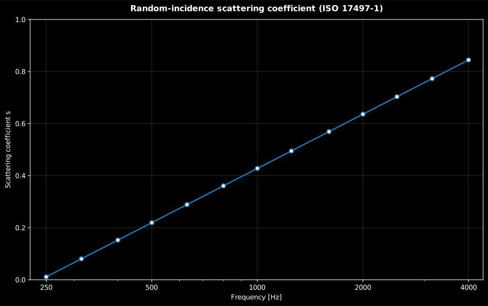*A random-incidence scattering coefficient rising with frequency as the surface roughness becomes comparable with the wavelength.* ### Directional diffusion coefficient (ISO 17497-2) ISO 17497-2:2012 measures, in the free field, how uniformly a surface spreads its reflected polar response over $n$ microphones. The autocorrelation-based coefficient (clause 8.1, Formula 5) is $$ d_\theta = \frac{\left( \sum_i p_i \right)^2 - \sum_i p_i^2}{(n - 1) \sum_i p_i^2}, \qquad p_i = 10^{L_i/10}, $$ 1 for a perfectly uniform response and tending to 0 for a single specular lobe; Formula 6 is the area-weighted form with $N_i = A_i / A_\mathrm{min}$ from the Formula 8 solid-angle factors ($A_i = (4\pi/\Delta\phi) \sin^2(\Delta\theta/4)$ at the zenith). Normalizing against a flat reference reflector of the same size removes edge diffraction (clause 8.2, Formula 7): $d_{\theta,\mathrm{n}} = (d_\theta - d_{\theta,\mathrm{r}})/(1 - d_{\theta,\mathrm{r}})$. The random-incidence value averages the source angles with weights 1:3:3:3:3 for 0°, ±30°, ±60° (clause 8.4). Anchors: the model-predicted 37-receiver arc of the published six-period $N = 7$ QRD (Cox & D'Antonio 3rd ed., Appendix B; Hargreaves et al. 2000, Table I) at 1000 Hz gives $d_\theta = 0.1099$, its flat reference $0.0049$ and $d_{\theta,\mathrm{n}} = 0.1055$; the band-averaged model predictions match the published Appendix B BEM normalised diffusion in the 200-400 Hz bands within 0.01 (a low-band anchor: the broadband 100-5000 Hz mean absolute deviation is about 0.09); zenith area factor 1.5710. *The object the coefficient is computed from, in the presentation clause 8.5 prescribes: one polar response per one-third-octave band and source position, on a semicircular plot with a decibel radial axis. This is the six-period $N = 7$ quadratic-residue diffuser of the anchor below, at 1 kHz. Its energy sits in a fan of discrete grating lobes rather than in one specular lobe, which is why $d_\theta$ is 0.11 where the flat reference of the same size scores 0.005, and why it is still nowhere near 1: the numerator rewards an even response, and a comb of lobes is not even.* See the [Diffusers guide](https://docs.jmrp.io/phonometry/materials/diffusers/diffusers/) for usage. ## In-situ road surface absorption (ISO 13472-1, ISO 13472-2) ISO 13472-1:2002 (extended surface method) recovers the normal-incidence absorption of a road surface in place, from one microphone above it: the direct and reflected components of an impulse response are separated by the **subtraction technique** and the **Adrienne window** (clause 6.4: a sharp leading edge, a mandated 5 ms flat top and a Blackman-Harris trailing edge), and $$ \alpha(f) = 1 - \frac{1}{K_\mathrm{r}^2} \left| \frac{H_\mathrm{r}(f)}{H_\mathrm{i}(f)} \right|^2, \qquad K_\mathrm{r} = \frac{d_\mathrm{s} - d_\mathrm{m}}{d_\mathrm{s} + d_\mathrm{m}} = \frac{2}{3} $$ for the mandatory geometry $d_\mathrm{s} = 1.25$ m, $d_\mathrm{m} = 0.25$ m (clause 4.2, Annex C); $K_\mathrm{r}$ is the spherical-spreading ratio between the direct and the image path. Ratioing the road measurement against one on a highly reflective reference surface cancels the entire electro-acoustic chain along with $K_\mathrm{r}$ (Annex B). The 5 ms window bounds the sampled area (Annex A closed form: radius ≈ 1.34 m for the standard geometry) and the valid range is 250 Hz – 4 kHz in one-third octaves. ISO 13472-2:2010 (spot method, 250–1600 Hz) instead couples a small impedance tube to the surface and defers the mathematics to the ISO 10534-2 transfer-function method below (its clauses 4/5.7/6.6); the implementation reuses that module, adding the Part 2 geometry and validity limits ($f_\mathrm{u} = 0.58\ c_0/d$; microphone spacing bounds $0.45\ c_0/f_\mathrm{max}$ and $0.05\ c_0/f_\mathrm{min}$, clause 5.4) and the Annex A subtractive correction for internal system losses. See the [In-situ Road-Surface Absorption guide](https://docs.jmrp.io/phonometry/materials/surfaces/road-absorption/) for usage. 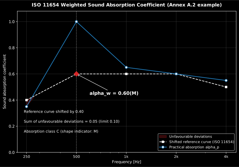## Acoustic material characterisation (ISO 11654, ISO 9053-1/2, ISO 10534-1/2, ASTM E2611) ### Weighted sound absorption (ISO 11654) ISO 11654:1997 condenses an ISO 354 third-octave absorption curve into a single number. The practical coefficient $\alpha_\mathrm{p}$ averages the three thirds of each octave 250 Hz – 4 kHz and rounds to steps of 0.05 (clause 4.1). The reference curve (0.80, 1.00, 1.00, 1.00, 0.90 at 250–4000 Hz) is then shifted downward in 0.05 steps until the sum of unfavourable deviations, counted only where the measurement falls *below* the shifted curve, is $\le 0.10$; $\alpha_\mathrm{w}$ is the shifted curve at 500 Hz (clause 4.2). A shape indicator flags excess absorption $\ge 0.25$ above the shifted curve: L at 250 Hz, M at 500/1000 Hz, H at 2000/4000 Hz (clause 4.3), and the informative Annex B maps $\alpha_\mathrm{w}$ to the absorption classes A–E. Because every quantity is a multiple of 0.05, the implementation does the whole grid arithmetic in integer twentieths, making the shift search and class boundaries exact and float-safe. The two Annex A worked examples are reproduced: $\alpha_\mathrm{p} = (0.35, 0.70, 0.65, 0.60, 0.55)$ → $\alpha_\mathrm{w} = 0.60$, class C; and raising 500 Hz to 1.00 keeps $\alpha_\mathrm{w} = 0.60$ but adds the indicator, "0.60(M)". *The ISO 11654 rating: practical absorption against the shifted reference, with the unfavourable deviation shaded and the weighted coefficient read at 500 Hz.* See the [Sound Absorption Measurement and Rating guide](https://docs.jmrp.io/phonometry/materials/absorbers/absorption-measurement/) for usage. ### Airflow resistance (ISO 9053-1/2) Airflow resistivity $\sigma = R\,A/d$ is the key transport parameter of a porous absorber. ISO 9053-1:2018 (static method) drives a steady flow through the specimen and fits $\Delta p = a\,u + b\,u^2$ through the origin (clause 7.5); since $R_\mathrm{s} = \Delta p / u = a + b\,u$, the linear coefficient is the zero-velocity specific resistance, reported at the reference velocity $u = 0.5$ mm/s. ISO 9053-2:2020 (alternating method) replaces the flowmeter with a ~2 Hz piston and a microphone in a closed cavity (clause 8.7, Formula 2): *The fit, and the single abscissa it is read at. The curve is slightly super-linear because the $b\,u^2$ term is real, but the reported quantity is the linear coefficient $a$ (the fit extrapolated back to zero velocity), evaluated at the 0.5 mm/s reference velocity, which is why the reference velocity has to be stated with any resistivity that is quoted.* $$ R = \kappa'\ \frac{p_\mathrm{s}}{2 \pi f V}\ \frac{h_\mathrm{t}}{h_\mathrm{s}}\ 10^{(L_{p\mathrm{s}} - L_{p\mathrm{t}})/20} $$ Only a level *difference* enters, so the sound-level device needs no absolute calibration. The effective exponent $\kappa'$ (Annex A, Formula A.7) corrects the adiabatic $\kappa$ for wall heat conduction through the thermal boundary layer $b = \sqrt{2 c_0 l_\mathrm{h} / \omega}$ (Formulae A.4/A.5). The Annex A.3 worked example (100 mm closed cylinder at 2 Hz: $b = 1.83$ mm, $\kappa' = 1.370 = 0.978\,\kappa$) is reproduced, and the validity guards of Formula 3 (transfer ratio < 0.3) and Formula 4 (10 dB background margin) are enforced. See the [Airflow Resistance guide](https://docs.jmrp.io/phonometry/materials/absorbers/airflow-resistance/) for usage. ### Impedance tube (ISO 10534-1, ISO 10534-2, ASTM E2611) A tube below its cut-on frequency ($f d < 0.58\ c_0$ circular, $< 0.50\ c_0$ rectangular; microphone-spacing limits $f s < 0.45\ c_0$ and $f > c_0/(20 s)$; clauses 4.2–4.5) carries only plane waves, so the surface reflection factor of a sample is fully observable. ISO 10534-2 (transfer-function method) compares the measured two-microphone transfer function $H_{12}$ with the analytic incident and reflected ones $H_\mathrm{I} = \mathrm{e}^{-j k_0 s}$, $H_\mathrm{R} = \mathrm{e}^{+j k_0 s}$ (Annex D) to give (clause 7, Eq. 17): $$ r = \frac{H_{12} - H_\mathrm{I}}{H_\mathrm{R} - H_{12}}\ \mathrm{e}^{2 j k_0 x_1}, \qquad \alpha = 1 - |r|^2, \qquad \frac{Z}{\rho c_0} = \frac{1 + r}{1 - r}, $$ with the complex wavenumber's attenuation lower bound $k_0'' = 1.94 \times 10^{-2} \sqrt{f}/(c_0 d)$ (Eq. A.18). ISO 10534-1 (standing-wave-ratio method) is the closed-form classic: $|r| = (s - 1)/(s + 1)$ from the max/min ratio $s = 10^{\Delta L/20}$ and the phase from the first-minimum position (Eqs. 12–26); an SWR of 3 gives exactly $|r| = 0.5$ and $\alpha = 0.75$. ASTM E2611-19 adds transmission: four microphones decompose the up- and downstream fields into the $A, B, C, D$ waves (Eqs. 17–20) and a two-load (or symmetric one-load) solve yields the specimen's 2×2 **transfer matrix** $[p; u]_0 = T\,[p; u]_d$ (Eqs. 16/22–24), from which the anechoic-backing normal-incidence transmission loss is (Eqs. 25/26) $$ TL = 20 \log_{10} \frac{\left| T_{11} + T_{12}/\rho c + \rho c\ T_{21} + T_{22} \right|}{2}, $$ plus the hard-backed reflection $R = (T_{11} - \rho c\,T_{21})/(T_{11} + \rho c\,T_{21})$ (Eq. 27), the material wavenumber $\arccos(T_{11})/d$ (Eq. 29) and the characteristic impedance $\sqrt{T_{12}/T_{21}}$ (Eq. 30). The three standards deliberately keep their own sign ansatz and temperature units (ISO in kelvin, ASTM in Celsius), and near-singular load solves raise a warning. Since neither standard prints a numeric example, the oracles are physics identities: the analytic air-layer matrix ($\det T = 1$, $T_{11} = T_{22}$, $TL = 0\ \text{dB}$, hard-backed $|R| = 1$), synthetic round-trips that recover a known $r$, and two-load recovery of an asymmetric reciprocal specimen. *What the ISO 10534-2 formula returns: $\alpha$ and $|r|$ for a 50 mm porous absorber over the working band of a 100 mm tube. The two curves are the same information ($\alpha = 1 - |r|^2$), so the figure is really one measurement drawn twice, and the rise with frequency is the layer thickness growing against the wavelength.* *The same four-pole entries answering two different questions: how much sound the free-standing layer lets through (the transmission loss above) and how much the same layer absorbs once it is backed rigidly. A material can be a good absorber and a poor barrier at once, which this pair makes plain.* See the [Impedance Tube guide](https://docs.jmrp.io/phonometry/materials/absorbers/impedance-tube/) for usage. ## References - Cox, T. J., & D'Antonio, P. (2017). *Acoustic absorbers and diffusers: Theory, design and application* (3rd ed.). CRC Press. ISBN 978-1-4987-4099-9. [doi:10.1201/9781315369211](https://doi.org/10.1201/9781315369211). Absorber and diffuser measurement and design, by the authors behind the ISO 17497-2 diffusion-coefficient method. - Allard, J. F., & Atalla, N. (2009). *Propagation of sound in porous media: Modelling sound absorbing materials* (2nd ed.). Wiley. ISBN 978-0-470-74661-5. [doi:10.1002/9780470747339](https://doi.org/10.1002/9780470747339). The porous-material theory linking the airflow-resistance and impedance-tube quantities of the characterisation section. - International Organization for Standardization. (2004). *Acoustics — Sound-scattering properties of surfaces — Part 1: Measurement of the random-incidence scattering coefficient in a reverberation room* (ISO 17497-1:2004+A1:2014, the edition implemented here). [iso.org catalogue](https://www.iso.org/standard/31397.html). The turntable scattering-coefficient method and its Annex A uncertainty chain. - International Organization for Standardization. (2012). *Acoustics — Sound-scattering properties of surfaces — Part 2: Measurement of the directional diffusion coefficient in a free field* (ISO 17497-2:2012). [iso.org catalogue](https://www.iso.org/standard/55293.html). The free-field directional diffusion coefficient and its solid-angle area weighting. - International Organization for Standardization. (1998). *Acoustics — Determination of sound absorption coefficient and impedance in impedance tubes — Part 2: Transfer-function method* (ISO 10534-2:1998; adopted in Europe as EN ISO 10534-2:2001; since revised as [ISO 10534-2:2023](https://www.iso.org/standard/81294.html)). [iso.org catalogue](https://www.iso.org/standard/22851.html). The two-microphone transfer-function method of the impedance-tube section. - ASTM International. (2019). *Standard test method for normal incidence determination of porous material acoustical properties based on the transfer matrix method* (ASTM E2611-19, the edition implemented here; since revised as [ASTM E2611-24](https://store.astm.org/e2611-24.html)). [ASTM store](https://store.astm.org/e2611-19.html). The four-microphone transfer-matrix decomposition and its transmission loss. - International Organization for Standardization. (2018). *Acoustics — Determination of airflow resistance — Part 1: Static airflow method* (ISO 9053-1:2018). [iso.org catalogue](https://www.iso.org/standard/69869.html). The static airflow-resistance method and its reference velocity.