Source: https://docs.jmrp.io/phonometry/reference/theory/environment-transport/ # Theory: Environment and Transport This page collects the theory behind outdoor and environmental noise: the whole-day rating descriptors and the impulsive-sound adjustment, atmospheric absorption, the general outdoor propagation method, occupational noise exposure with its uncertainty budget, and the sound power determination methods. It is part of the [theory reference](https://docs.jmrp.io/phonometry/reference/theory/). 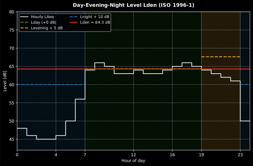## Environmental descriptors (ISO 1996-1) The **day-evening-night level** $L_\mathrm{den}$ (ISO 1996-1:2016, 3.6.4) is an energy average over the 24 h day with penalty weightings of **+5 dB for the evening** and **+10 dB for the night**: $$ L_\mathrm{den} = 10 \log_{10}\left\lbrace\frac{1}{24}\left[ t_\mathrm{d}\ 10^{0.1 L_\mathrm{day}} + t_\mathrm{e}\ 10^{0.1 (L_\mathrm{evening} + 5)} + t_\mathrm{n}\ 10^{0.1 (L_\mathrm{night} + 10)} \right]\right\rbrace $$ with default period durations $(t_\mathrm{d}, t_\mathrm{e}, t_\mathrm{n}) = (12, 4, 8)$ h; countries may define the periods differently (3.6.4 Note 1). The **day-night level** $L_\mathrm{dn}$ (3.6.5) drops the evening period: $$ L_\mathrm{dn} = 10 \log_{10}\left\lbrace\frac{1}{24}\left[ t_\mathrm{d}\ 10^{0.1 L_\mathrm{day}} + t_\mathrm{n}\ 10^{0.1 (L_\mathrm{night} + 10)} \right]\right\rbrace, \qquad (t_\mathrm{d}, t_\mathrm{n}) = (15, 9)\ \text{h} $$ Both are special cases of the **composite whole-day rating level** (6.5, generalizing Formulae 5–6), where each period $i$ contributes its rating level $L_i$ plus an adjustment $K_i$, weighted by its share of the day: $$ L_\mathrm{R} = 10 \log_{10}\left[ \sum_i \frac{h_i}{24}\ 10^{0.1 (L_i + K_i)} \right], \qquad \sum_i h_i = 24\ \text{h} $$ The adjustments $K_i$ cover time-of-day penalties (ISO 1996-1 Table A.1: evening 5 dB, night 10 dB) as well as source-character adjustments (e.g. tonal penalties), which the ECMA-418-1 TNR/PR assessments can justify objectively. *A 24-hour $L_\mathrm{Aeq}$ profile split into day, evening and night, the +5/+10 dB penalties and the resulting $L_\mathrm{den}$.* See the [Environmental levels guide](https://docs.jmrp.io/phonometry/environment/assessment/environmental-levels/) for usage. ## Impulsive-sound prominence (NT ACOU 112) An impulse annoys beyond its energy, so environmental surveys after ISO 1996-2 penalize periods containing prominent impulsive sounds; NT ACOU 112:2002 makes that penalty objective. From the A-weighted, time-weighting-F level history of a single event, the onset rate (dB/s) and the level difference (dB) of the onset (which qualifies when steeper than 10 dB/s, clauses 4.5–4.7) predict the perceived prominence (clause 7, Formula 1): $$ P = 3 \log_{10}(\text{onset rate}) + 2 \log_{10}(\text{level difference}), $$ designed to peak around 15 for very sudden, loud impulses. The adjustment to the measurement-period level takes the governing (highest-$P$) impulse (clause 8, Formula 2): $$ K_\mathrm{I} = 1.8\ (P - 5)\ \text{dB} \quad (P > 5;\ \text{else } K_\mathrm{I} = 0), $$ and the whole-day rating level combines the adjusted periods energetically (clause 8, Note 1): $$ L_{\mathrm{Ar},T} = 10 \log_{10}\Big[ \frac{1}{T} \sum_N \Delta t_N\ 10^{(L_{\mathrm{Aeq},N} + K_{\mathrm{I},N})/10} \Big]. $$ $K_\mathrm{I}$ is exactly the kind of source-character adjustment that enters the ISO 1996-1 composite rating level above. The anchors $P(1000\ \text{dB/s}, 30\ \text{dB}) = 9 + 2\log_{10} 30 = 11.95$ and $K_\mathrm{I}(P{=}10) = 9.0$ dB are reproduced exactly. *Both inputs of $P$ are geometry on this trace, which is why the method needs a level history and not a level. The onset rate is the slope of the fitted line through the rise, in dB/s, and the qualifying threshold of 10 dB/s is a steepness on this axis; the level difference is the height of the same rise. Three strikes are detected here and only the steepest-and-tallest one governs the adjustment.* See the [Impulse Prominence guide](https://docs.jmrp.io/phonometry/environment/assessment/impulsive-sound/) for usage. ## Outdoor propagation and occupational exposure (ISO 9613-1/2, ISO 9612) ### Atmospheric absorption (ISO 9613-1) Air is a lossy medium: a propagating tone loses energy to shear viscosity and heat conduction (classical and rotational losses, growing as $f^2$) and to the **vibrational relaxation** of the oxygen and nitrogen molecules, each an energy reservoir that resonates near a humidity- and temperature-dependent relaxation frequency. ISO 9613-1:1993, Eq. (5) gives the pure-tone attenuation coefficient $\alpha$ in decibels per metre: $$ \alpha = 8.686\ f^2 \Big[ 1.84\times10^{-11} \big(p_\mathrm{a}/p_\mathrm{r}\big)^{-1} \big(T/T_0\big)^{1/2} + \big(T/T_0\big)^{-5/2} \big( 0.01275\ \tfrac{\mathrm{e}^{-2239.1/T}}{f_\mathrm{rO} + f^2/f_\mathrm{rO}} + 0.1068\ \tfrac{\mathrm{e}^{-3352.0/T}}{f_\mathrm{rN} + f^2/f_\mathrm{rN}} \big) \Big], $$ with the oxygen and nitrogen relaxation frequencies $f_\mathrm{rO}$, $f_\mathrm{rN}$ of Eq. 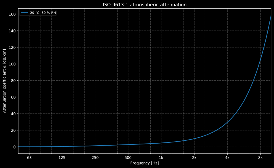(3)/(4), the reference conditions $T_0 = 293.15$ K, $p_\mathrm{r} = 101.325$ kPa (Clause 4.2) and the molar water-vapour concentration $h$ from the relative humidity (Annex B). At low frequency $\alpha \propto f^2$; near each relaxation frequency the corresponding term peaks and rolls off, which is why $\alpha$ rises by two decades from 50 Hz to 10 kHz and why raising the humidity sweeps a peak across the band. The library reproduces Table 1 to under 0.4 % (the standard's own printed precision), well inside its stated $\pm 10$ %; passing `exact_midband=True` snaps each frequency onto the exact midbands $f_\mathrm{m} = 1000 \cdot 10^{k/10}$ (Note 5) used to compute that table. The same $\alpha$ is the only route to the ISO 354 power attenuation coefficient $m = \alpha/(10 \log_{10} e)$, exposed as `air_attenuation_m`. *The ISO 9613-1 coefficient for the 20 °C, 50 % relative-humidity reference atmosphere: the $f^2$ rise spans two decades from 50 Hz to 10 kHz.* *The humidity claim of the paragraph above, drawn: four atmospheres, and a spread far wider than the $\pm 10$ % claimed for any one of them. At 2 kHz the coefficient is 9.9 dB/km at the 20 °C / 50 % reference and **45.5 dB/km** at the same temperature and 10 % humidity, a factor 4.6 from humidity alone, worth 36 dB over a kilometre. Note which way it goes: drying the air *increases* the mid-band attenuation, because the oxygen relaxation frequency falls with humidity and drags its peak down into the band. Temperature moves the curves far less: 0 °C at 70 % and 20 °C at 50 % differ by 0.02 dB/km at 1 kHz.* ### Outdoor propagation, general method (ISO 9613-2) ISO 9613-2:1996 predicts the octave-band level at a receiver **downwind** of a point source (or the equivalent moderate temperature inversion) as $L_{fT}(DW) = L_W + D_\mathrm{c} - A$ (Eq. (3)), where $D_\mathrm{c}$ is the directivity correction and $A$ is the octave-band attenuation, a sum of independent physical mechanisms (Eq. (4)): $$ A = A_\mathrm{div} + A_\mathrm{atm} + A_\mathrm{gr} + A_\mathrm{bar} + A_\mathrm{misc}. $$ The library implements the four general terms of Clause 7; the informative $A_\mathrm{misc}$ (foliage, industrial sites, housing) and reflections are left to the caller. **Geometrical divergence** is spherical spreading from a point source, $A_\mathrm{div} = 20 \log_{10}(d/d_0) + 11$ dB with $d_0 = 1$ m (Eq. (7)): exactly 51 dB at 100 m, +6 dB per distance doubling. **Atmospheric absorption** is $A_\mathrm{atm} = \alpha\ d$ (Eq. (8)) with $\alpha$ the ISO 9613-1 coefficient above. **Ground effect** $A_\mathrm{gr} = A_\mathrm{s} + A_\mathrm{r} + A_\mathrm{m}$ (Eq. (9)) sums a source, receiver and middle region, each evaluated from the Table 3 functions $a'/b'/c'/d'$ and its ground factor $G$ (0 hard, 1 porous); a negative $A_\mathrm{gr}$ denotes a net gain from the ground reflection. An alternative A-weighted-only form $A_\mathrm{gr} = 4.8 - (2 h_\mathrm{m}/d)[17 + 300/d] \ge 0$ (Eq. (10)) is offered for porous ground when only the A-weighted level matters, paired with the solid-angle index $D_\Omega$ (Eq. (11)). **Screening** by a barrier is the diffraction insertion loss $$ D_z = 10 \log_{10}\big[ 3 + (C_2/\lambda)\ C_3\ z\ K_\mathrm{met} \big] \quad\text{dB}, $$ (Eq. (14)) with $C_2 = 20$ (or 40 when ground reflections are handled by image sources), $C_3 = 1$ for a single edge or Eq. (15) for a double edge, the path-length difference $z = d_\mathrm{ss} + d_\mathrm{sr} - d$ (Eq. (16)/(17)), wavelength $\lambda = 340/f$ and the meteorological factor $K_\mathrm{met}$ (Eq. (18)); $D_z$ is capped at 20 dB (single) or 25 dB (double). For a top-edge barrier the ground effect of the screened path is folded into the screening term, $A_\mathrm{bar} = D_z - A_\mathrm{gr} \ge 0$ (Eq. (12), Note 13); for a lateral (vertical-edge) barrier $A_\mathrm{bar} = D_z$ and the ground term is kept (Eq. (13)). The long-term average level subtracts the meteorological correction $C_\mathrm{met}$ (Eq. (6), (21)/(22)). The method's stated accuracy is $\pm 1$ to $\pm 3$ dB for broadband noise up to 1000 m (Table 5). *The four terms at their true relative sizes, band by band, for a 200 m path over porous ground with a 4 m barrier. $A_\mathrm{div}$ is 57 dB in every band because it is pure geometry. $A_\mathrm{atm}$ is nothing at 63 Hz and 18.7 dB at 8 kHz, so it is the term that decides how far high frequencies travel and no other. $A_\mathrm{gr}$ is where the low bands live and is **negative** at 63 Hz (−4.6 dB: the ground reflection adds energy rather than removing it). $A_\mathrm{bar}$ is at its 20 dB cap from 2 kHz up but falls to zero at 250 Hz, because the top-edge form subtracts the ground effect the screened path gives away, $A_\mathrm{bar} = D_z - A_\mathrm{gr} \geq 0$, and 250 Hz is exactly where $A_\mathrm{gr}$ peaks. Which term is worth refining depends entirely on the band and the geometry.* ### Occupational noise exposure and uncertainty (ISO 9612) ISO 9612:2009 is the engineering method (accuracy grade 2) for a worker's daily noise exposure level $L_\mathrm{EX,8h}$, normalised to a nominal 8 h day. Three **measurement strategies** trade effort for representativeness. The *task-based* method (Clause 9) splits the day into tasks, energy-averages $I \ge 3$ samples per task (Eq. 7) and sums the task contributions $L_{\mathrm{EX,8h},m} = L_{p,\mathrm{A,eq}T,m} + 10 \log_{10}(T_m/T_0)$ energetically (Eq. 9/10). The *job-based* method (Clause 10) energy-averages $N \ge 5$ random samples over a homogeneous exposure group (Eq. 11) and normalises the effective-day duration (Eq. 12); the *full-day* method (Clause 11) does the same arithmetic on whole-day measurements (Eq. 13). The **Annex C** uncertainty budget is normative. The combined standard uncertainty is $u^2 = \sum c_i^2 u_i^2$ (C.1) and the expanded uncertainty is $U = k\ u$ with $k = 1.65$ for a **one-sided** 95 % interval (Clause 14), so the reported upper limit is $L_\mathrm{EX,8h} + U$. The task and job methods differ in an instructive way: the task noise-sampling uncertainty $u_{1\mathrm{a}}$ divides the summed squared deviations by $I(I-1)$ (the standard error of the mean, Eq. C.6) whereas the job/full-day sampling uncertainty $u_1$ is the plain sample standard deviation with denominator $N-1$ (Eq. C.12), so the same spread contributes more in the job method (fewer, coarser samples). The task budget (Eq. C.3) adds the sensitivity coefficients $c_{1\mathrm{a}}$ (Eq. C.4) and $c_{1\mathrm{b}}$ (Eq. C.5) and an optional task-duration uncertainty $u_{1\mathrm{b}}$ (Eq. C.7); the job/full-day budget (Eq. C.9) reads $c_1 u_1$ from Table C.4 as a function of $(N, u_1)$ and adds the instrument uncertainty $u_2$ (Table C.5) and microphone-position uncertainty $u_3 = 1.0$ dB in quadrature. Peak levels $L_{p,\mathrm{Cpeak}}$ are reported without an uncertainty: Annex C provides no method for them (Table C.5, Note 1). The three worked examples of Annexes D (task, $L_\mathrm{EX,8h} = 84.3$ dB, $U = 2.7$ dB), E (job, $88.1$ dB, $3.8$ dB) and F (full-day, $90.1$ dB, $3.4$ dB) are reproduced to the standard's printed precision: every intermediate of Annex E is digit-exact, and its final level differs only by the standard's own pre-rounding of the effective-day level (see the [Occupational Noise Exposure guide](https://docs.jmrp.io/phonometry/perception/hearing/occupational-exposure/)). *What the budget buys: the Annex D worked day, its three task contributions, the energy-summed $L_\mathrm{EX,8h}$ and the band up to $L_\mathrm{EX,8h} + U$ that the one-sided 95 % interval adds on top. The reported result is the pair, not the line, and with $U = 2.7$ dB the upper limit sits 2.7 dB above the number, which is enough to cross an action value on its own.* See the [Outdoor Propagation guide](https://docs.jmrp.io/phonometry/environment/propagation/outdoor-propagation/) and the [Occupational Noise Exposure guide](https://docs.jmrp.io/phonometry/perception/hearing/occupational-exposure/) for usage. ## Sound power determination (ISO 3744/3745/3746, ISO 3741, ISO 9614-1/2/3) The sound power level $L_W = 10 \log_{10}(P/P_0)$ ($P_0 = 1$ pW) is an *emission* quantity: unlike a pressure level it does not depend on the receiver distance or the room. Three families of methods recover it, one per measured quantity: a **sound pressure** over an enveloping surface (ISO 3744/3746, and ISO 3745 when the room is anechoic) or in a diffuse field (ISO 3741), a **sound intensity** held at discrete points (ISO 9614-1) or scanned over that same surface (ISO 9614-2 and ISO 9614-3), and the **surface velocity** of the radiating casing, which takes no acoustic measurement at all: ISO/TS 7849, whose radiation factor is the radiation efficiency derived in the [vibration reference](https://docs.jmrp.io/phonometry/reference/theory/vibration/#point-mobilities-and-radiation-efficiency-cremer-5-hopkins-29). 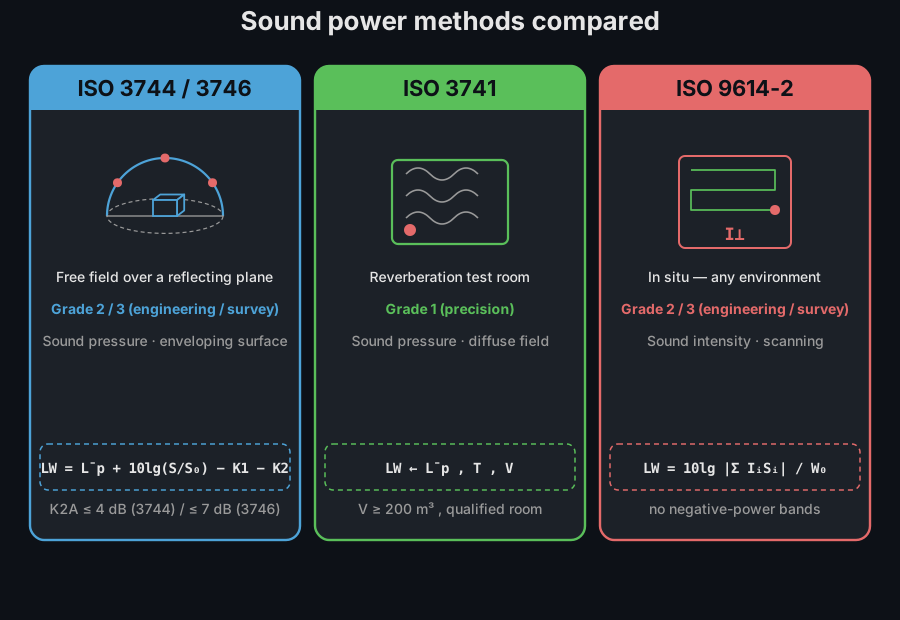*The seven routes to $L_W$, one row per measured quantity: a sound pressure, a sound intensity, or the surface velocity of the casing.* ### Enveloping-surface pressure (ISO 3744/3746) Over a reflecting plane the free-field relation is simply $L_W = \bar{L}_p + 10 \log_{10}(S/S_0)$: the mean-square pressure averaged over an enveloping surface of area $S$, multiplied by $S$, is the radiated power. Two corrections restore that idealisation. Uncorrelated **background noise** adds its mean square to the source's, so with the margin $\Delta L_p = L_\mathrm{ST} - L_\mathrm{bg}$ the source-only level is recovered by subtracting $K_1 = -10 \log_{10}(1 - 10^{-\Delta L_p/10})$ (from $p_\mathrm{src}^2 = p_\mathrm{ST}^2 (1 - 10^{-\Delta L_p/10})$). The **reverberant field** of a non-anechoic room adds a near-uniform energy density $4P/(A c)$ to the direct $P/(S c)$, so the surface level exceeds the free-field value by their ratio, $K_2 = 10 \log_{10}(1 + 4 S/A)$, with $A$ the room's equivalent absorption area. The surface area is the closed form of the geometry: a hemisphere $S = 2 \pi r^2$ over one reflecting plane (halved and quartered for two and three planes), a one-plane box $S = 4(ab + bc + ca)$ with $a = 0.5\ l_1 + d$, $b = 0.5\ l_2 + d$, $c = l_3 + d$. ISO 3746 (survey) shares the maths with looser criteria. The expanded uncertainty is $U = 2 \sqrt{\sigma_{R0}^2 + \sigma_\mathrm{omc}^2}$. ### Precision grade in anechoic rooms (ISO 3745) ISO 3745:2012 is the grade-1 (precision) sibling: a qualified anechoic or hemi-anechoic room removes the reverberant field, so there is no $K_2$ term and the corrections become meteorological. The power level is $L_W = \bar{L}_p + 10 \log_{10}(S/S_0) + C_1 + C_2 + C_3$ (Eq. 14/15) over a full sphere $S = 4 \pi r^2$ or hemisphere $S = 2 \pi r^2$, with the background correction $K_{1i} = -10 \log_{10}(1 - 10^{-0.1 \Delta L_{pi}})$ applied per microphone position *before* the energy average (Eq. 11); no correction is needed above a 15 dB margin, and below 10 dB (250 Hz – 5 kHz) or 6 dB (edge bands) the correction is clamped and the result flagged as an upper bound (clause 9.4.2). The meteorological terms are $C_1 = -10 \log_{10}(p_\mathrm{s}/p_{\mathrm{s}0}) + 5 \log_{10}[(273 + \theta)/\theta_0]$ and $C_2 = -10 \log_{10}(p_\mathrm{s}/p_{\mathrm{s}0}) + 15 \log_{10}[(273 + \theta)/\theta_1]$ with $\theta_0 = 314$ K, $\theta_1 = 296$ K: at the 23 °C / 101.325 kPa reference $C_2 = 0$ exactly and $C_1 = -0.128$ dB; and $C_3 = A_0 (1.0053 - 0.0012 A_0)^{1.6}$ with $A_0 = a(f)\ r$ restores the ISO 9613-1 air absorption over the measurement radius. The Annex D/E microphone arrays are built in as digit-exact coordinate tables (40 equal-area positions; the mirror set 21–40 is added when the band-SPL spread exceeds $N_\mathrm{M}/2$, clause 9.3.2), and the same positions yield the directivity index $DI_i = L_{pi} - \bar{L}_p$ (Eq. 21). The clause 10.5 uncertainty example, $U = 2\sqrt{0.5^2 + 2.0^2} = 4.12$ dB, is reproduced, along with the Table 2/3 per-band $\sigma_{R0}$ values. ### Reverberation room (ISO 3741) In a qualified diffuse field the steady energy density $w = 4P/(A c)$ ties the power to the room absorption, giving $L_W = \bar{L}_p + 10 \log_{10}(A/A_0) - 6$ plus higher-order corrections, with $A = (55.26/c)(V/T_{60})$ and $c = 20.05 \sqrt{273 + \theta}$. The **Waterhouse correction** $10 \log_{10}(1 + S c/(8 V f))$ compensates the extra energy stored in the boundary layer that interior microphones miss ($S c/(8 V f) = S \lambda/(8 V)$, so it fades as frequency rises); the $4.34\ A/S$ term is the mean-free-path air correction, and $C_1$, $C_2$ carry the result to the reference meteorological conditions (23 °C, 101.325 kPa). The **comparison method** subtracts a reference source of known power measured in the same room, $L_W = L_{W(\text{RSS})} + (\bar{L}_p - \bar{L}_{p,\text{RSS}} + C_2)$, so the absorption-area, Waterhouse and $C_1$ terms cancel and the room need not be characterised. ### Discrete-point intensity (ISO 9614-1) Part 1 holds the probe still. One position stands for each segment of the measurement surface, so the partial power is $P_i = I_{\mathrm{n}i} S_i$ (Eq. 11) and the sound power is $L_W = 10 \log_{10}(\sum_i P_i / P_0)$ (Eq. 12). That sum is printed without the absolute-value bars of the general definition because clause 9.2 disposes of the negative case instead: a band whose $\sum_i P_i$ comes out negative is outside the method rather than a band with a level to report. One segment carrying negative power is ordinary, and is what $F_3$ exists to quantify. What separates Part 1 from a scan is not the integral but what decides whether it was sampled finely enough, and with a fixed set of positions the surface has to answer that itself. The Annex A indicators average over positions without area weighting: $F_1$ is the temporal variability (Eq. A.1), $F_2 = L_p - L_{|I_\mathrm{n}|}$ and $F_3 = L_p - L_{I_\mathrm{n}}$ are the reactivity and recirculation indicators (Eqs. A.3 to A.7), and $F_4 = \frac{1}{|\overline{I_\mathrm{n}}|} \sqrt{\sum_i (I_{\mathrm{n}i} - \overline{I_\mathrm{n}})^2 / (N - 1)}$ is the field non-uniformity (Eqs. A.8 and A.9), which is Part 1's own. Annex B turns it into a position count: criterion 2 asks $N > C F_4^2$ (Eq. B.2) with $C$ from Table B.2, so a surface that radiates unevenly demands more positions, band by band, and the grade a band earns is the grade whose $C$ that inequality still satisfies. Criterion 1, $L_\mathrm{d} > F_2$ (Eq. B.1), puts the probe against the field before any of that, and no amount of averaging rescues a band that fails it. The gate figure in the next subsection is drawn in exactly these names, because they are Part 1's. ### Intensity scanning (ISO 9614-2) Sound intensity is the net energy flux $\vec{I} = \overline{p\ \vec{u}}$, so by the divergence theorem the power through a closed surface is $P = \sum_i \langle I_{\mathrm{n},i} \rangle\ S_i$. A steady source *outside* the surface contributes zero net flux (its energy enters and leaves), which is why intensity rejects stationary background noise, but it can still drive a band's $P$ negative, in which case that band is not determinable. Two normative field indicators gate validity: the surface pressure-intensity indicator $F_{pI} = [L_p] - L_W + 10 \log_{10}(S/S_0)$ (reactivity) and the negative-partial-power indicator $F_{+/-} = 10 \log_{10}(\sum_i \lvert P_i \rvert / \lvert \sum_i P_i \rvert)$ (recirculation), together with the probe's dynamic capability $L_\mathrm{d} = \delta_{pI0} - K$ ($K = 10$ dB grade 2, 7 dB grade 3), which must exceed $F_{pI}$. A band earns the engineering grade when $L_\mathrm{d} > F_{pI}$, $F_{+/-} \le 3$ dB and the two repeated sweeps agree within the Table 2 limit. *The gate as a picture rather than an inequality, drawn here in the ISO 9614-1 naming, $F_2$ for what Part 2 calls $F_{pI}$. The reactivity indicator climbs towards low frequency and crosses the dynamic-capability line at 125 Hz: that band fails, and no amount of averaging will rescue it, because the cause is the field near the surface and not the analyser. $F_3$ rising above $F_2$ in the same band reveals inward-flowing partial intensity, and the $F_4$ bars set how many positions the surface needs.* ### Precision intensity scanning (ISO 9614-3) ISO 9614-3:2002 upgrades the scanning method to precision grade with a tighter indicator machinery. The partial powers $P_i = I_{\mathrm{n},i} S_i$ (Eq. 5) sum as before, but validity now rests on the signed and unsigned pressure-intensity indicators $F_{pI_\mathrm{n}} = \bar{L}_p - L_{I\mathrm{n}}$ (Eqs. B.3/B.6, the F2/F3 of ISO 9614-1) and the normalized intensity non-uniformity $F_\mathrm{S}$ (Eq. B.8), through five acceptance criteria (Annex C): scan repeatability $|L_{I\mathrm{n}}(1) - L_{I\mathrm{n}}(2)| \le s/2$ (C.1), dynamic capability $L_\mathrm{d} = \delta_{pI0} - K \ge F_{pI_\mathrm{n}}(\text{signed})$ with the precision bias-error factor $K = 10$ dB (C.2), $F_{pI_\mathrm{n}}(\text{signed}) - F_{pI_\mathrm{n}}(\text{unsigned}) \le 3$ dB (C.3), $F_\mathrm{S} \le 2$ (C.4) and the scan-density convergence $0.83 \le F_\mathrm{S}(1)/F_\mathrm{S}(2) \le 1.2$ (C.5). Eq. 10 normalizes the result to the reference meteorological conditions, $L_{W0} = L_W - 15 \log_{10}[(B/101325) \cdot 296.15/(273.15 + \theta)]$. Bands whose net power is negative are not determinable (clause 9.2) and are flagged. A uniform normal intensity recovers the power exactly (100 µW over 3.75 m² → 80.0 dB re 1 pW), independent of how the surface is segmented. See the [Sound Power guide](https://docs.jmrp.io/phonometry/devices/emission/sound-power/) for usage. ## References - Salomons, E. M. (2001). *Computational atmospheric acoustics*. Kluwer Academic Publishers. ISBN 978-1-4020-0390-5. [doi:10.1007/978-94-010-0660-6](https://doi.org/10.1007/978-94-010-0660-6). The wave-based outdoor propagation theory behind the engineering approximations of the ISO 9613-2 section. - Attenborough, K., & Van Renterghem, T. (2021). *Predicting outdoor sound* (2nd ed.). CRC Press. [doi:10.1201/9780429470806](https://doi.org/10.1201/9780429470806). The ground impedance and meteorological effects underlying the ground-effect and barrier terms. - Maekawa, Z. (1968). Noise reduction by screens. *Applied Acoustics*, 1(3), 157-173. [doi:10.1016/0003-682X(68)90020-0](https://doi.org/10.1016/0003-682X(68)90020-0). The screen-attenuation chart that the barrier insertion-loss formulas descend from. - Fahy, F. J. (1995). *Sound intensity* (2nd ed.). E&FN Spon. ISBN 978-0-419-19810-9. [doi:10.4324/9780203475386](https://doi.org/10.4324/9780203475386). The intensity physics behind the scanning methods: active intensity and the p-p error budget. - International Organization for Standardization. (2016). *Acoustics — Description, measurement and assessment of environmental noise — Part 1: Basic quantities and assessment procedures* (ISO 1996-1:2016). [iso.org catalogue](https://www.iso.org/standard/59765.html). The composite rating level and Table A.1 adjustments of the descriptors section. - Nordtest. (2002). *Acoustics: Prominence of impulsive sounds and for adjustment of LAeq* (Nordtest Method NT ACOU 112). [nordtest.info](https://www.nordtest.info/wp/2002/05/01/acoustics-prominence-of-impulsive-sounds-and-for-adjustment-of-laeq-nt-acou-112/). The onset-rate prominence and LAeq adjustment of the impulsive-sound section. - International Organization for Standardization. (2022). *Acoustics — Description, measurement and assessment of environmental noise — Part 3: Objective method for the measurement of prominence of impulsive sounds and for adjustment of LAeq* (ISO/PAS 1996-3:2022). [iso.org catalogue](https://www.iso.org/standard/77035.html). The ISO successor built on the NT ACOU 112 prominence. - International Organization for Standardization. (1993). *Acoustics — Attenuation of sound during propagation outdoors — Part 1: Calculation of the absorption of sound by the atmosphere* (ISO 9613-1:1993). [iso.org catalogue](https://www.iso.org/standard/17426.html). The pure-tone attenuation coefficient and its relaxation physics. - International Organization for Standardization. (1996). *Acoustics — Attenuation of sound during propagation outdoors — Part 2: General method of calculation* (ISO 9613-2:1996; revised in 2024, the 1996 method is the implemented one). [iso.org catalogue](https://www.iso.org/standard/20649.html). The attenuation chain (divergence, air, ground, barrier) of the general-method section. - International Organization for Standardization. (2009). *Acoustics — Determination of occupational noise exposure — Engineering method* (ISO 9612:2009). [iso.org catalogue](https://www.iso.org/standard/41718.html). The three measurement strategies and the Annex C uncertainty budget of the occupational section. - International Organization for Standardization. (2010). *Acoustics — Determination of sound power levels and sound energy levels of noise sources using sound pressure — Engineering methods for an essentially free field over a reflecting plane* (ISO 3744:2010). [iso.org catalogue](https://www.iso.org/standard/52055.html). The enveloping-surface method with its background and reverberant-field corrections. - International Organization for Standardization. (2012). *Acoustics — Determination of sound power levels and sound energy levels of noise sources using sound pressure — Precision methods for anechoic rooms and hemi-anechoic rooms* (ISO 3745:2012). [iso.org catalogue](https://www.iso.org/standard/45362.html). The precision anechoic method with its meteorological corrections and microphone arrays. - International Organization for Standardization. (2010). *Acoustics — Determination of sound power levels and sound energy levels of noise sources using sound pressure — Precision methods for reverberation test rooms* (ISO 3741:2010). [iso.org catalogue](https://www.iso.org/standard/52053.html). The diffuse-field method with the Waterhouse correction and the comparison method. - International Organization for Standardization. (1993). *Acoustics — Determination of sound power levels of noise sources using sound intensity — Part 1: Measurement at discrete points* (ISO 9614-1:1993). [iso.org catalogue](https://www.iso.org/standard/17427.html). The field indicators and dynamic-capability criterion shared by the intensity-scanning methods.