Source: https://docs.jmrp.io/phonometry/perception/speech/speech-transmission/ # Speech Transmission Index (IEC 60268-16) A public-address system, an intercom, a reverberant lecture hall: each is a *transmission channel* between a talker's mouth and a listener's ear, and each degrades speech in its own way. The **Speech Transmission Index** (STI) of IEC 60268-16 rates that channel with a single number in $[0, 1]$ by measuring how much of the speech *envelope* survives the trip. This page covers the modulation-transfer physics behind the index, the indirect method from a measured room impulse response, and the direct STIPA measurement with its standardized test signal. > [!NOTE] > **STI vs SII.** The STI characterises a *transmission channel* (how much of > the speech modulation a room or sound system preserves) while the SII > predicts intelligibility from *audibility*: how much of the speech spectrum > clears the noise and the hearing threshold at the listener's ear. For the > latter, see the [Speech Intelligibility Index guide](https://docs.jmrp.io/phonometry/perception/speech/speech-intelligibility/). ## 1. The modulation transfer function Reverberation and noise do not muffle speech uniformly; they blur its *envelope*: the slow (0.63–12.5 Hz) intensity modulations that carry syllables. STI quantifies how much of that modulation survives from mouth to ear, per octave band, as the **modulation transfer function** $m(F)$. A delta-like channel keeps $m = 1$ (STI = 1); reverberation low-passes the envelope following Schroeder's closed form, and steady noise scales it: $$ m(F) = \frac{1}{\sqrt{1 + \left(2\pi F\,\frac{T_{60}}{13.8}\right)^2}} \cdot \frac{1}{1 + 10^{-\mathrm{SNR}/10}} $$ Modulation *depth* is the thing worth measuring because intelligibility rides on the depth of the envelope valleys, not on the loudness of the peaks. A talker alternates energy bursts (vowels) with near-silences (stop gaps, fricative onsets) at syllable rate, and a listener segments speech by hearing those dips. A reverberant tail fills the dips from behind, since late energy smears into the gaps; steady noise raises their floor. In both cases the received modulation depth shrinks, and with it the contrast between speech sounds, even when the average level barely changes. The full method probes $m(F)$ at 14 modulation frequencies (0.63 Hz to 12.5 Hz in one-third-octave steps) in each of the 7 octave bands from 125 Hz to 8 kHz, converts each $m$ to an effective signal-to-noise ratio clipped to ±15 dB, and combines the results, band-weighted, into the index: the STI is an effective SNR of the *envelope*, mapped onto $[0, 1]$.

Show the code for this figure

```python import numpy as np import matplotlib.pyplot as plt from phonometry import speech fs = 48000 # STI vs reverberation time: sweep speech.sti_from_impulse_response over synthetic # exponential decays (white noise x exp(-6.9077 t / T60)) at a T60 grid, # exactly the physics behind the curve above: rng = np.random.default_rng(0) t60_grid = np.array([0.3, 0.5, 0.8, 1.2, 1.6, 2.0, 2.5, 3.0, 4.0, 5.0]) sti_values = [] for t60 in t60_grid: t = np.arange(int(2 * t60 * fs)) / fs ir = rng.standard_normal(t.size) * np.exp(-6.9077 * t / t60) sti_values.append(speech.sti_from_impulse_response(ir, fs).sti) fig, ax = plt.subplots() ax.semilogx(t60_grid, sti_values, "o-") ax.set_xlabel("Reverberation time T60 [s]") ax.set_ylabel("STI") ax.set_ylim(0.0, 1.0) ax.grid(True, which="both", alpha=0.3) plt.show() ```

## 2. Indirect and direct (STIPA) measurement ```python import numpy as np from phonometry import speech fs = 48000 # A measured room impulse response (synthesized decay so the example runs) ir = np.random.default_rng(0).standard_normal(fs) * np.exp(-6.9 * np.arange(fs) / fs / 0.5) # Indirect method: from a measured room impulse response res = speech.sti_from_impulse_response(ir, fs, snr=25.0) print(f"STI = {res.sti:.2f} ({res.rating})") # e.g. 0.62 (D) # Direct STIPA measurement: play speech.stipa_signal() in the room, record it test = speech.stipa_signal(fs, seconds=18.0, level_db=80.0) recording = test # in practice, the microphone signal after playback res = speech.stipa(recording, fs) res.plot() # per-band modulation transfer index (MTI) bars, STI + rating in the title ``` Whichever route produced it, the result is worth reading band by band before the single number is quoted: the STI is a weighted combination of seven octave-band modulation transfer indices, and a room usually fails in a particular part of the spectrum rather than uniformly.

Show the code for this figure

```python import numpy as np import matplotlib.pyplot as plt from phonometry import speech # A reverberant hall (T60 = 0.9 s) measured with a 15 dB speech-to-noise # ratio: a synthesized exponential decay stands in for the measured IR. fs = 48000 rng = np.random.default_rng(0) n = np.arange(fs) ir = rng.standard_normal(fs) * np.exp(-6.9078 * n / fs / 0.9) res = speech.sti_from_impulse_response(ir, fs, snr=15.0) print(round(res.sti, 3), res.rating) # 0.583 E # One line: the per-band MTI bars with the STI and its rating in the title. res.plot() plt.show() # By hand, mirroring what STIResult.plot() draws: bands = [125, 250, 500, 1000, 2000, 4000, 8000] fig, ax = plt.subplots() ax.bar(np.arange(len(bands)), res.mti) ax.set_xticks(np.arange(len(bands))) ax.set_xticklabels([f"{b}" for b in bands]) ax.set_xlabel("Frequency [Hz]") ax.set_ylabel("Modulation transfer index MTI") ax.set_ylim(0.0, 1.0) ax.set_title(f"STI = {res.sti:.2f} (rating {res.rating})") plt.show() ```

In this hall the seven indices sit within 0.06 of each other, the signature of a decay that is uniform across the spectrum plus a broadband noise floor. A profile that sags at 125 Hz and 250 Hz instead points at low-frequency reverberation (too little bass absorption), while one that falls only at 4 kHz and 8 kHz usually means the loudspeaker is out of the listener's direct-sound coverage, since air and directivity strip the top bands first. Those are different remedies, and only the per-band view distinguishes them. 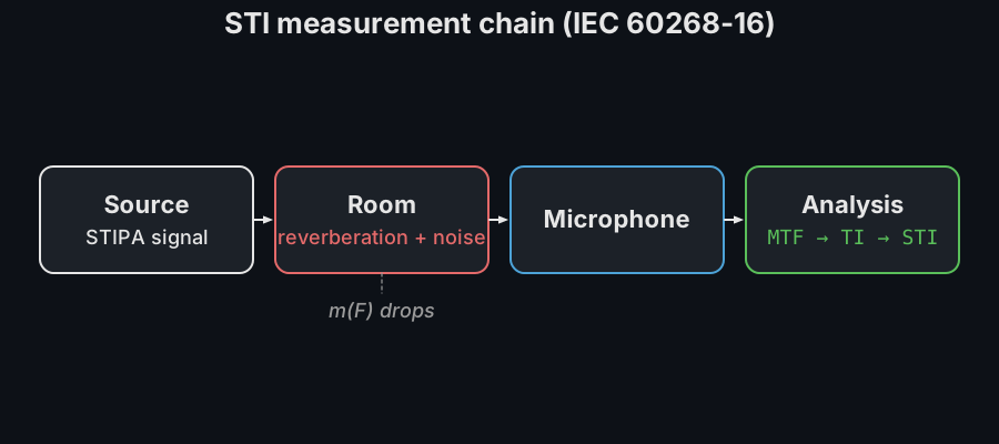The direct measurement sends the STIPA signal along the full chain drawn below, from the source through the room to the microphone and into the per-band modulation analysis that yields the index. `stipa` emits a `UserWarning` when the recording is shorter than the recommended 15 s (IEC 60268-16 STIPA practice, 15 s to 25 s): below that the slow modulation components are averaged over too few periods and the STI is biased low (an ideal loopback gives STI ≈ 0.956 at 5 s vs ≈ 0.998 at 18 s). The implementation follows **Edition 5 (2020)**: Edition 4's normative PDF is the base and every Ed. 5 change is source-attributed in the code; the only numeric delta is the revised male speech spectrum of clause A.6.1. That male spectrum is the only one there is: Edition 5 removed the female speech option (foreword, item d), so its absence here is the standard's, not the library's. CI checks the standard's own verification vectors: the six weighting-factor band pairs to ±0.001 STI, the $m$ ↔ STI mapping table, the level-dependent masking control points, and Schroeder-form decays at four $T_{60}$ values. The analyzer is also verified end to end against the **IEC 60268-16 rev 5 verification test bench** signals from [stipa.info](https://www.stipa.info) (Embedded Acoustics BV): the direct-method modulation-depth staircase (Annex C.3.2), the indirect-method exponential decays against the closed-form Schroeder MTF (C.3.3), the filter-bank slope test with a +41 dB unmodulated adjacent-octave tone (C.4.2, $m \ge 0.5$), the weighting-factor band pairs (A.2.2) and the filter-bank phase-distortion test with half-octave edge carriers (A.3.1.2, |STI bias| < 0.01 over TI = 0.1–0.9). All five suites pass with the level-dependent features disabled, as the bench prescribes. The 49 certified WAVs stay local (third-party data, not committed); CI re-derives the same signal constructions synthetically in the conformance suite. ### Direct or indirect: choosing between them Each route has failure modes the standard is explicit about: - **Non-linear or time-variant channels.** The indirect method assumes a linear, time-invariant channel: an impulse response cannot represent clipping, compressors, automatic gain control or a vocoder. For a sound system with non-linear processing in the chain, measure directly: the STIPA signal at least travels through the real chain, and the FULL STI signal is the reliable choice where the distortion is severe (IEC 60268-16 clause 6.3 and Table 3). That 14-modulation-frequency direct test signal is not implemented here, though: the library provides the STIPA direct signal (`stipa_signal`/`stipa`) and the indirect full-STI computation from an impulse response only. - **Level-dependent effects.** The STI is not level-invariant: auditory masking and the reception threshold act on the *absolute* band levels at the listener. Play the test signal at the system's operating level (the standard's Annex J practice sets it 3 dB above the $L_\mathrm{Aeq}$ of continuous speech at the position) and pass `levels=` and `ambient=` so the analysis includes them; an impulse response measured loud and rescaled afterwards misses these effects entirely. Section 3 moves a measurement made at one level and noise condition to another. - **Impulsive and fluctuating background noise.** A dropped tool or babble during a direct measurement corrupts the measured modulation depths (clause 7.13). The standard's remedy is the indirect route: average the impulse response with MLS or sweeps for a noise-free MTF, then add the noise degradation back via `snr=` or `levels=`/`ambient=`. A quick sanity check is to run the analyzer with the source off; the residual STI should stay below 0.20. - **Statistical spread.** The STIPA signal is pseudo-random noise, so repeated direct measurements scatter by up to about 0.03 STI even in steady conditions (and more in fluctuating noise); repeat and compare rather than trusting a single run, and respect the minimum duration flagged by the `UserWarning` above. ### `sti_from_impulse_response()` / `stipa()` parameters | Parameter | Type | Units | Range / default | Notes | | :--- | :--- | :--- | :--- | :--- | | `ir` / `x` | 1D array | any / Pa | non-empty | IR (indirect) or STIPA recording (direct) | | `fs` | int | Hz | > 0 | | | `snr` | float or 7-vector, optional | dB | default `None` | Adds steady-noise degradation | | `levels` | 7-vector, optional | dB SPL | default `None` | Enables auditory masking + reception threshold (Tables A.2/A.3) | | `ambient` | 7-vector, optional | dB SPL | needs `levels` | Ambient noise band levels | | `reference` | 1D array, optional (`stipa`) | — | default `None` | Measured source signal instead of the nominal $m = 0.55$ | Both return `STIResult`: `sti`, `mti` (7 bands), `mtf` (7×14 or 7×2), `band_levels` and `ambient_levels` (the two spectra the corrections used, and what section 3 reads to move the result to another condition), `rating` (Annex F letter `A+`…`U`). ### IEC 60268-16 report (`.report()`) `STIResult.report(path)` renders a one-page PDF fiche laid out like a voice-alarm / public-address intelligibility verification report: a standard-basis line stating the measurement method (the full STI indirect method from an impulse response, or the direct STIPA method on a recorded signal), an optional metadata header block, a per-octave-band modulation transfer index table beside the per-band MTI bars (the result's own `.plot()`), the boxed `STI = X` single number with the Annex F qualification band, an optional verdict row and a footer with the fixed disclaimer. It uses the same `ReportMetadata` container (documented under [Insulation ratings](https://docs.jmrp.io/phonometry/buildings/insulation/insulation-ratings/#report-metadata-reportmetadata)) and rendering engine as the ISO 717 insulation fiche; a supplied `requirement` is read as the minimum required STI (a higher STI passes). Rendering needs reportlab and, for the figure the fiche embeds, matplotlib (`pip install "phonometry[report,plot]"`); only `engine="reportlab"` is supported. Pass `language="es"` for a Spanish fiche. ```python from phonometry import ReportMetadata, speech res = speech.sti_from_impulse_response(ir, fs) res.report( "sti_fiche.pdf", metadata=ReportMetadata( specimen="Concourse voice-alarm loudspeaker line", measurement_standard="IEC 60268-16", laboratory="Phonometry Reference Laboratory", requirement=0.5, # minimum required STI (a higher STI passes) ), ) ``` The example fiche, regenerated with `make reports`, is kept rendered in the repository. Click the preview to open the PDF: [](https://raw.githubusercontent.com/jmrplens/phonometry/main/.github/reports/iec60268_16_sti_example.pdf) *Speech transmission index fiche (`STIResult.report`), STI with the Annex F band.* ## 3. Occupancy noise and a different speech level A hall is measured out of hours, empty, with the test signal at whatever level the amplifier happened to be set to. The rating it has to meet is for the hall in use: an audience in the seats, and the announcement at its operational level. Annex M of IEC 60268-16 moves the measurement to that condition arithmetically, in four steps and without a second visit: 1. **Acquire.** The modulation transfer matrix as measured, with the noise, masking and threshold of the measurement still in it, together with the speech and background-noise octave-band levels present while it was made. 2. **Remove.** Divide out the correction those levels produce, stripping the background noise, the auditory masking of Table A.2 and the reception threshold of Table A.3 back out and leaving the transmission channel alone. 3. **Reapply.** Multiply by the correction the operational levels produce, putting the occupancy noise, masking and threshold of the simulated condition in. 4. **Process.** Run the resulting matrix through the A.5.4 to A.5.6 chain into the index. Taking the old condition out before putting the new one in is not ceremony, and it is not an approximation either. The measured matrix is a product of two things, and only one of them survives the move: the transmission channel, the room's decay and the system's response, is what the empty measurement and the occupied prediction have in common, while the noise, the masking and the threshold belong to the listening condition and go with it. Those three cannot be updated from how far the levels moved, either, because none of them is a function of the change. Auditory masking is a piecewise function of the *absolute* combined level of the band below, changing slope at 63 dB and again at 67 dB and 100 dB, and the reception threshold of Table A.3 is an absolute intensity that does not move at all. Both have to be re-derived at the new levels, and dividing the old correction out is what leaves something to derive them for. The shortcut the two steps exist to forbid is the tempting one: running the noise correction over the measured matrix again with the occupancy levels counts the noise twice, because the measurement's own noise is already in there. Note also where the truncation goes. The channel step 2 recovers can exceed 1.0 in a band whose correction was strong, and it is not clamped between the steps: the $m > 1$ truncation of A.5.3 NOTE 1 is for the matrix about to be processed, which is the one step 3 produces. The annex's own example never tests that, its recovered matrix peaking at 0.997, but a measurement whose correction bites harder would. For the library the two steps are also one piece of code, which is the other reason to keep them apart. Step 2 divides by the same clause A.5.3 factor a forward measurement multiplies by and step 3 multiplies by it, so the masking of Table A.2 and the threshold of Table A.3 have a single implementation and the adjustment cannot drift away from the measurement it adjusts. ```python import numpy as np from phonometry import speech # The reverberant hall of this section, measured empty: a 0,9 s decay at # 48 kHz stands in for the measured impulse response. fs = 48000 rng = np.random.default_rng(0) ir = rng.standard_normal(fs) * np.exp(-6.9078 * np.arange(fs) / fs / 0.9) # The Ed.5 male speech spectrum of clause A.6.1 at 68 dB overall, and the # empty hall's own ventilation noise, both in dB SPL per octave band. band_shape = np.array([-2.5, 0.5, 0.0, -6.0, -12.0, -18.0, -24.0]) speech_empty = band_shape - 10 * np.log10(np.sum(10 ** (band_shape / 10))) + 68.0 noise_empty = np.array([42.0, 36.0, 31.0, 28.0, 25.0, 23.0, 21.0]) empty = speech.sti_from_impulse_response( ir, fs, levels=speech_empty, ambient=noise_empty ) print(f"{empty.sti:.2f} ({empty.rating})") # 0.60 (D) # The audience in, and the announcement left where it was. noise_occupied = np.array([54.0, 50.0, 47.0, 44.0, 40.0, 35.0, 30.0]) occupied = empty.adjusted_for_levels( operational_levels=speech_empty, operational_ambient=noise_occupied ) print(f"{occupied.sti:.2f} ({occupied.rating})") # 0.56 (F) # The same room with the announcement 6 dB louder. louder = empty.adjusted_for_levels( operational_levels=speech_empty + 6.0, operational_ambient=noise_occupied ) print(f"{louder.sti:.2f} ({louder.rating})") # 0.59 (E) ``` The occupancy noise costs two rating letters, and six decibels more from the talker buys one of them back. That is the argument for doing this before the handover rather than after the complaint: the empty hall passed. `STIResult.adjusted_for_levels()` reads the measurement condition off the result, which is why it needs only the operational one and why it refuses a result computed without `levels=`: such a result carries at most the flat `snr=` noise factor, none of the level-dependent masking and threshold, and no spectra to re-derive them from, so dividing the full correction out would silently lower the answer. Where the matrix comes from somewhere else, `speech.sti_adjusted_for_levels()` takes all four spectra beside it. Every result the adjustment returns is an ordinary `STIResult`, so the per-band reading of section 2 applies to it, and it is worth taking. The single number says the hall lost two letters; the bands say where it lost them:

Show the code for this figure

```python import matplotlib.pyplot as plt import numpy as np from phonometry import speech fs = 48000 rng = np.random.default_rng(0) n = np.arange(fs) ir = rng.standard_normal(fs) * np.exp(-6.9078 * n / fs / 0.9) shape = np.array([-2.5, 0.5, 0.0, -6.0, -12.0, -18.0, -24.0]) talker = shape - 10 * np.log10(np.sum(10 ** (shape / 10))) + 68.0 empty_noise = np.array([42.0, 36.0, 31.0, 28.0, 25.0, 23.0, 21.0]) full_noise = np.array([54.0, 50.0, 47.0, 44.0, 40.0, 35.0, 30.0]) measured = speech.sti_from_impulse_response(ir, fs, levels=talker, ambient=empty_noise) occupied = measured.adjusted_for_levels( operational_levels=talker, operational_ambient=full_noise ) louder = measured.adjusted_for_levels( operational_levels=talker + 6.0, operational_ambient=full_noise ) # One line: the adjusted result is an STIResult, so it draws its own bars. occupied.plot() plt.show() # By hand, the three conditions on one band axis: positions = np.arange(7) fig, ax = plt.subplots() for i, res in enumerate((measured, occupied, louder)): ax.bar(positions + (i - 1) * 0.27, res.mti, width=0.27, label=f"STI {res.sti:.2f} ({res.rating})") ax.set_xticks(positions) ax.set_xticklabels(["125", "250", "500", "1k", "2k", "4k", "8k"]) ax.set_xlabel("Frequency [Hz]") ax.set_ylabel("Modulation transfer index MTI") ax.set_ylim(0.0, 0.95) ax.legend() plt.show() ```

The 125 Hz band gives up the most, because that is where the audience is loudest and the talker has least margin: about 7 dB of speech-to-noise there against 16 dB at 500 Hz. The extra 6 dB then gives back most where most was lost, nearly nine tenths of the 125 Hz loss against about half of the 1 kHz one. Neither of those is visible in the index. ### What the adjustment cannot tell you - **It moves the listening condition, not the room.** The channel step 2 recovers is carried through untouched, so nothing an audience does to the acoustics is in the answer. Bodies and clothing absorb: the occupied reverberation time is shorter than the empty one, and the occupied channel is in truth *better* than the one measured. An empty-hall measurement is pessimistic about the reverberation and optimistic about the noise, and this corrects only the second. Where the audience changes the absorption materially, the honest route is an impulse response for the occupied room, measured or predicted, with the adjustment applied to that. - **The operational speech level is an input, not a forecast.** The annex says what the STI would be if the talker or the amplifier delivered those band levels. Whether they will is a different question: a live talker lifts their voice in noise, a chain with a limiter or automatic gain control does not simply scale, and a system asked for 6 dB more may clip instead of delivering it, at which point it is no longer the linear channel the measured matrix stands for. - **The noise it models is steady.** Occupancy noise is babble, which fluctuates and, being speech-shaped, masks in ways an intensity added per octave band does not represent. The standard's caution about fluctuating noise (clause 7.13) applies to the condition being simulated as much as to the one being measured. - **The measurement's own spectra are what step 2 removes.** A wrong `measured_levels` or `measured_ambient` takes out the wrong correction, and step 3 has no way to notice; the adjusted matrix is then wrong in a direction nothing downstream reports. That is why `STIResult.adjusted_for_levels()` reads them off the result instead of asking again. - **It is still one listener position.** Every spectrum in it is the one at the microphone, so an occupancy-adjusted result answers for that seat and no other. ### `sti_adjusted_for_levels()` parameters | Parameter | Type | Units | Range / default | Notes | | :--- | :--- | :--- | :--- | :--- | | `mtf` | (7, n) array | — | ≥ 0, finite | The matrix as measured, noise and masking included; values above 1 are truncated to 1, and above 1.3 warn that the measurement is likely invalid (A.5.3 NOTE 1) | | `measured_levels` | 7-vector | dB SPL | required | Speech band levels during the measurement | | `measured_ambient` | 7-vector, optional | dB SPL | default `None` | Background-noise band levels during the measurement | | `operational_levels` | 7-vector | dB SPL | required | Speech band levels of the condition simulated | | `operational_ambient` | 7-vector, optional | dB SPL | default `None` | Occupancy-noise band levels of that condition | > [!IMPORTANT] > **Which edition this is.** What the library implements is the Edition 4 (2011) > Annex M procedure, verified against the printed intermediates of its Table M.1 > worked example rather than only against the STI it ends on: both 98-value MTF > matrices, every scalar row on the way to them, the effective SNRs, the band > MTI row and the index. The only prints not used as oracles are the step 4 > clamp and transmission-index matrices, which the annex derives from its own > rounded SNR print. The Edition 5 foreword says greater information is given > in Annex M about these adjustments (item g), and its table of contents grows > the annex from three printed pages to ten; the body of the Edition 5 annex > could not be obtained, so what those pages add beside this procedure is not > known here. ## See also - [Room Acoustics](https://docs.jmrp.io/phonometry/buildings/rooms/room-acoustics/): the measured impulse response the indirect method consumes, and the open-plan metrics (ISO 3382-3) built on per-position STI. - [Speech Intelligibility Index](https://docs.jmrp.io/phonometry/perception/speech/speech-intelligibility/): the audibility-based ANSI S3.5 index that complements the STI. - [Loudness](https://docs.jmrp.io/phonometry/perception/psychoacoustics/loudness/) and [Sound Quality Metrics](https://docs.jmrp.io/phonometry/perception/psychoacoustics/sound-quality/): loudness, sharpness, tonality and roughness of the received sound. - [Theory](https://docs.jmrp.io/phonometry/reference/theory/perception/): the modulation-transfer derivation and the $m$ ↔ STI mapping. - API reference: [`speech.sti`](https://docs.jmrp.io/phonometry/reference/api/speech/sti/). ## References - Houtgast, T., & Steeneken, H. J. M. (1985). A review of the MTF concept in room acoustics and its use for estimating speech intelligibility in auditoria. *The Journal of the Acoustical Society of America*, 77(3), 1069-1077. [doi:10.1121/1.392224](https://doi.org/10.1121/1.392224). The modulation-transfer framework of section 1 and the $m$ ↔ STI mapping the index is built on. ## Standards IEC 60268-16:2020 (Edition 5), *Sound system equipment — Part 16: Objective rating of speech intelligibility by speech transmission index*: the modulation transfer function and the $m$ ↔ STI mapping, the STIPA test signal and direct method, the indirect method from the impulse response, auditory masking and the reception threshold (Tables A.2/A.3), the revised male speech spectrum (clause A.6.1), the Annex F rating letters and, from the Edition 4 print, the Annex M adjustment of a measured result to occupancy noise and another speech level.