Source: https://docs.jmrp.io/phonometry/environment/propagation/outdoor-propagation/ # Outdoor Sound Propagation Predicting the noise a distant source delivers to a receiver outdoors is a book-keeping exercise: start from the source **sound power** and subtract, band by band, every mechanism that attenuates the sound on its way: spherical spreading, the air itself, the ground, and any barrier in between. This page covers the two parts of ISO 9613 that supply those terms: **ISO 9613-1**, the pure-tone atmospheric absorption coefficient $\alpha$, and **ISO 9613-2**, the general method that assembles $\alpha$ with divergence, ground and screening into an octave-band prediction. The atmospheric coefficient also closes the loop with room acoustics, since ISO 354 defers its air power-attenuation coefficient $m$ entirely to $\alpha$. ## 1. Atmospheric absorption (ISO 9613-1) Air is not lossless. A propagating tone bleeds energy into shear viscosity and heat conduction (the *classical and rotational* losses that grow as $f^2$) and into the **vibrational relaxation** of the oxygen and nitrogen molecules, each an energy store that resonates near a humidity- and temperature-dependent relaxation frequency. ISO 9613-1:1993, Eq. (5) collects all of this into the pure-tone attenuation coefficient $\alpha$, in decibels per metre: $$ \alpha = 8.686\ f^2 \Big[ 1.84\times10^{-11} \big(p_\mathrm{a}/p_\mathrm{r}\big)^{-1} \big(T/T_0\big)^{1/2} + \big(T/T_0\big)^{-5/2} \big( 0.01275\ \tfrac{\mathrm{e}^{-2239.1/T}}{f_\mathrm{rO} + f^2/f_\mathrm{rO}} + 0.1068\ \tfrac{\mathrm{e}^{-3352.0/T}}{f_\mathrm{rN} + f^2/f_\mathrm{rN}} \big) \Big], $$ with the oxygen and nitrogen relaxation frequencies $f_\mathrm{rO}$, $f_\mathrm{rN}$ (Eq. (3)/(4)), the reference conditions $T_0 = 293.15$ K and $p_\mathrm{r} = 101.325$ kPa (Clause 4.2), and the molar water-vapour concentration $h$ obtained from the relative humidity by the Annex B psychrometric conversion. Two features dominate the shape: at low frequency $\alpha \propto f^2$, so it rises steeply; and near each relaxation frequency the matching term peaks and rolls off. Between them $\alpha$ climbs about two decades from 50 Hz to 10 kHz, and, because humidity sets $f_\mathrm{rO}$, sweeping the humidity moves a relaxation peak across the band, so the driest air is not always the least absorbing. *The dry 20 °C / 10 % curve absorbs most at mid frequencies, but the humid curves overtake it below ~200 Hz: the relaxation signature.*

Show the code for this figure

```python import matplotlib.pyplot as plt import numpy as np from phonometry import environment freqs = np.geomspace(50.0, 10000.0, 400) fig, ax = plt.subplots() for temp, rh in [(20.0, 50.0), (20.0, 10.0), (0.0, 70.0), (30.0, 80.0)]: ax.loglog(freqs, environment.air_attenuation(freqs, temperature_c=temp, relative_humidity_percent=rh) * 1000.0, label=f"{temp:g} °C, {rh:g} % RH") ax.set_xlabel("Frequency [Hz]") ax.set_ylabel("Attenuation coefficient alpha [dB/km]") ax.legend() plt.show() ```

```python import numpy as np from phonometry import environment bands = [63, 125, 250, 500, 1000, 2000, 4000, 8000] # octave-band centres [Hz] # Pure-tone attenuation coefficient alpha [dB/m] at 20 °C, 50 % RH, one atmosphere alpha = environment.air_attenuation(bands, temperature_c=20.0, relative_humidity_percent=50.0) print(np.round(alpha * 1000.0, 2)) # in dB/km, as Table 1 tabulates # [ 0.12 0.44 1.31 2.73 4.66 9.89 29.67 105.29] # Reproduce an ISO 9613-1 Table 1 cell exactly (10 °C, 70 %, 1 kHz) cell = environment.air_attenuation(1000.0, temperature_c=10.0, relative_humidity_percent=70.0, exact_midband=True) * 1000.0 print(round(float(cell), 2)) # 3.66 (dB/km, Table 1) # Feed real conditions into the ISO 354 power attenuation coefficient m [1/m] m = environment.air_attenuation_m([1000.0, 4000.0], temperature_c=20.0, relative_humidity_percent=50.0) print(np.round(m, 5)) # [0.00107 0.00683] ``` `air_attenuation` returns dB/m (Table 1 prints dB/km, i.e. $\times 1000$); it is fully vectorized over `frequencies` with scalar temperature, humidity and pressure. Passing `exact_midband=True` snaps each requested frequency onto the exact one-third-octave midband $f_\mathrm{m} = 1000 \cdot 10^{k/10}$ (Eq. (6), Note 5) used to compute Table 1, so the library reproduces every tabulated point to under 0.4 %, the standard's own three-significant-figure precision, far inside its stated $\pm 10$ % accuracy (Clause 7.1). Inputs outside the tabulated ranges (−20…+50 °C, 10…100 % RH, 50…10 000 Hz, or above the 200 kPa validity envelope) still compute but raise an `AtmosphericAbsorptionWarning`; non-physical inputs (non-positive frequency, humidity outside 0…100 %, sub-absolute-zero temperature) raise `ValueError`. `air_attenuation_m` composes $\alpha$ with the ISO 354 conversion $m = \alpha/(10 \log_{10} e)$ so an ISO 354 caller can feed real atmospheric conditions straight into `absorption_area` / `absorption_coefficient` instead of hand-entering $m$. ### `air_attenuation()` / `air_attenuation_m()` parameters | Parameter | Type / shape | Units | Range / default | Notes | | :--- | :--- | :--- | :--- | :--- | | `frequencies` | scalar or 1D array | Hz | > 0 | Vectorized; 50–10 000 Hz tabulated | | `temperature_c` | float | °C | default `20.0` | −20…+50 tabulated; outside warns | | `relative_humidity_percent` | float | % | default `50.0` | 10…100 tabulated; `[0, 100]` allowed | | `atmospheric_pressure_kpa` | float | kPa | default `101.325` | ≤ 200 valid (Clause 7); above warns | | `exact_midband` | bool | — | default `False` | Snap to $f_\mathrm{m} = 1000\cdot10^{k/10}$ (reproduces Table 1) | `air_attenuation` returns $\alpha$ in dB/m; `air_attenuation_m` returns $m = \alpha/(10 \log_{10} e)$ in 1/m for ISO 354. ### A plottable result: `atmospheric_attenuation()` For a figure or a quick look, `atmospheric_attenuation()` wraps the same coefficient in a small `AtmosphericAttenuation` result. 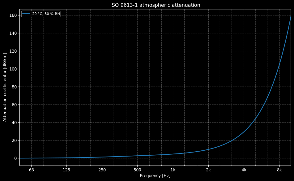It carries the frequency grid, the coefficient $\alpha$ and the atmospheric conditions, and exposes `.plot()` for the classic $\alpha$-versus-frequency curve (drawn in dB/km, the Table 1 unit, on a linear ordinate over a logarithmic frequency axis). Passing a `distance` also records the total attenuation $A = \alpha\,d$, in decibels, over that path as `total_attenuation`, the ISO 9613-2 $A_\mathrm{atm}$ of Eq. (8). ```python from phonometry import environment res = environment.atmospheric_attenuation( [63, 125, 250, 500, 1000, 2000, 4000, 8000], temperature_c=20.0, relative_humidity_percent=50.0, ) res.plot() # alpha in dB/km against frequency (needs matplotlib) ``` *On a linear decibel ordinate the coefficient stays near zero up to about 1 kHz and then climbs steeply, passing 20 dB/km near 3 kHz and reaching over 150 dB/km by 10 kHz at the reference 20 °C / 50 % RH atmosphere.*

Show the code for this figure

```python import matplotlib.pyplot as plt import numpy as np from phonometry import environment # One line: the coefficient curve straight from the result. res = environment.atmospheric_attenuation( np.geomspace(50.0, 10000.0, 400), temperature_c=20.0, relative_humidity_percent=50.0, ) res.plot() plt.show() # Or by hand from air_attenuation (dB/m, so scale by 1000 for dB/km): freqs = np.geomspace(50.0, 10000.0, 400) fig, ax = plt.subplots() ax.semilogx(freqs, environment.air_attenuation(freqs, temperature_c=20.0, relative_humidity_percent=50.0) * 1000.0) ax.set_xlabel("Frequency [Hz]") ax.set_ylabel("Attenuation coefficient alpha [dB/km]") plt.show() ```

## 2. General method of calculation (ISO 9613-2) ISO 9613-2:1996 predicts the octave-band level at a receiver **downwind** of a point source (or under the equivalent moderate temperature inversion, Clause 5). The equivalent-continuous downwind level is $$ L_{fT}(DW) = L_W + D_\mathrm{c} - A, \qquad A = A_\mathrm{div} + A_\mathrm{atm} + A_\mathrm{gr} + A_\mathrm{bar} + A_\mathrm{misc}, $$ (Eq. (3)/(4)) where $L_W$ is the octave-band sound power level, $D_\mathrm{c}$ the directivity correction (directivity index plus a solid-angle index $D_\Omega$), and $A$ the total attenuation. The library implements the four general terms of Clause 7; the informative $A_\mathrm{misc}$ (foliage, industrial sites, housing; Annex A) and reflections off vertical obstacles (Clause 7.5) are **not implemented**: the standard treats them as informative and they are left to the caller. The geometry of the screening term fixes the vocabulary: the diffraction edge splits the source-to-receiver distance into $d_\mathrm{ss}$ and $d_\mathrm{sr}$, and the extra path length over the edge is $z = d_\mathrm{ss} + d_\mathrm{sr} - d$. When the line of sight passes *above* the top edge, the standard gives $z$ a negative sign (`Barrier(line_of_sight_clear=True)`) and Eq. (14) still applies with $K_\mathrm{met} = 1$: $D_z$ falls continuously from $10 \log_{10} 3 \approx 4.8$ dB at grazing incidence to zero as the clearance deepens, never below zero. ### The four attenuation terms * **Geometrical divergence** $A_\mathrm{div} = 20 \log_{10}(d/d_0) + 11$ dB, $d_0 = 1$ m (Eq. (7)): spherical spreading from a point source. Exactly 51 dB at 100 m, +6 dB per distance doubling. The $+11$ ($= 10 \log_{10} 4\pi$) sets the level at the 1 m reference distance. * **Atmospheric absorption** $A_\mathrm{atm} = \alpha\ d$ (Eq. (8)) with $\alpha$ the ISO 9613-1 coefficient, negligible at low frequency and dominant at 8 kHz over long paths. $\alpha$ is evaluated at the *exact* base-10 midband behind each nominal band label (7 943.3 Hz for "8 kHz"), the convention behind the ISO 9613-2 Table 2 coefficients (the nominal-frequency evaluation runs ~1.3 % high at 8 kHz). The ISO 9613-2 functions default to 20 °C and 70 % relative humidity (one of the Table 2 reference atmospheres the standard tabulates) while `air_attenuation` itself defaults to the ISO 9613-1 usual 50 %. * **Ground effect** $A_\mathrm{gr} = A_\mathrm{s} + A_\mathrm{r} + A_\mathrm{m}$ (Eq. (9)) sums a source, receiver and middle region, each from the Table 3 functions $a'/b'/c'/d'$ and its ground factor $G$ (0 = hard/reflective, 1 = porous/absorbing). A **negative** $A_\mathrm{gr}$ is a net *gain* from constructive ground reflection. * **Screening** by a barrier is the diffraction insertion loss $D_z = 10 \log_{10}\big[ 3 + (C_2/\lambda)\ C_3\ z\ K_\mathrm{met} \big]$ (Eq. (14)), capped at 20 dB (single edge) or 25 dB (double edge). For a top-edge barrier the ground effect of the screened path folds into it, $A_\mathrm{bar} = D_z - A_\mathrm{gr} \ge 0$ (Eq. (12), Note 13); for a lateral barrier $A_\mathrm{bar} = D_z$ and the ground term is retained (Eq. (13)). `outdoor_propagation_attenuation` assembles the four terms into an `OutdoorAttenuation` result whose per-band arrays sum, band by band, to `a_total`, so the divergence, atmospheric, ground and barrier contributions stay separable. The stacked breakdown makes the frequency character obvious: the barrier helps most at high frequency (short wavelength) until it saturates at the cap, atmospheric absorption bites only at 8 kHz, and the ground dip lives in the mid bands.

Show the code for this figure

```python import matplotlib.pyplot as plt import numpy as np from phonometry import environment bands = np.array([63.0, 125.0, 250.0, 500.0, 1000.0, 2000.0, 4000.0, 8000.0]) barrier = environment.Barrier(source_to_edge=101.0, edge_to_receiver=101.0) att = environment.outdoor_propagation_attenuation( 200.0, source_height=1.5, receiver_height=1.5, frequencies=bands, ground_source=1.0, ground_middle=1.0, ground_receiver=1.0, barrier=barrier, temperature_c=15.0, relative_humidity_percent=70.0, ) # One line — the same stacked breakdown with the total overlaid: att.plot() # By hand: x = np.arange(len(bands)) fig, ax = plt.subplots() # Separate positive and negative baselines: a negative term (Agr is a net # gain at 63 Hz here) stacks below zero, and the signed heights sum to a_total. pos_bottom = np.zeros(len(bands)) neg_bottom = np.zeros(len(bands)) for term, label in [(att.a_div, "Adiv — divergence"), (att.a_atm, "Aatm — atmospheric"), (att.a_gr, "Agr — ground"), (att.a_bar, "Abar — barrier")]: ax.bar(x, term, bottom=np.where(term >= 0.0, pos_bottom, neg_bottom), label=label) pos_bottom += np.maximum(term, 0.0) neg_bottom += np.minimum(term, 0.0) ax.plot(x, att.a_total, "D-", color="black", label="A — total") ax.set_xticks(x) ax.set_xticklabels([f"{b:g}" for b in bands]) ax.set_xlabel("Octave-band centre frequency [Hz]") ax.set_ylabel("Attenuation A [dB]") ax.legend() plt.show() ```

```python import numpy as np from phonometry import environment bands = [63, 125, 250, 500, 1000, 2000, 4000, 8000] # octave-band centres [Hz] # A point source and receiver 1.5 m high, 200 m apart over porous ground # (G = 1), screened midway by a barrier that raises the path over its top edge # (dss = dsr ~ 101 m). Geometry feeds the pathlength-difference equations. barrier = environment.Barrier(source_to_edge=101.0, edge_to_receiver=101.0) att = environment.outdoor_propagation_attenuation( 200.0, source_height=1.5, receiver_height=1.5, frequencies=bands, ground_source=1.0, ground_middle=1.0, ground_receiver=1.0, barrier=barrier, temperature_c=15.0, relative_humidity_percent=70.0, ) print(np.round(att.a_div, 1)) # [57. 57. 57. 57. 57. 57. 57. 57.] divergence print(np.round(att.a_gr, 2)) # [-4.65 2.34 13.79 9.76 1.3 -0. -0. -0. ] print(np.round(att.a_bar, 2)) # [13.78 8.89 0. 6.69 18.01 20. 20. 20. ] print(np.round(att.a_total, 1)) # [66.2 68.3 71. 73.9 77.1 78.8 82.3 95.8] att.plot() # the stacked breakdown above (needs matplotlib) # Predicted receiver level from an octave-band sound power Lw = 95 dB lw = np.full(len(bands), 95.0) lp = environment.predicted_receiver_level( lw, environment.PropagationGeometry(200.0, 1.5, 1.5), # d, hs, hr frequencies=bands, ground=environment.GroundFactors(1.0, 1.0, 1.0), # Gs, Gm, Gr barrier=barrier, atmosphere=environment.AtmosphericConditions( temperature_c=15.0, relative_humidity_percent=70.0), ) print(np.round(lp, 1)) # [28.8 26.7 24. 21.1 17.9 16.2 12.7 -0.8] ``` `predicted_receiver_level` composes $L_{fT}(DW) = L_W + D_\mathrm{c} - A$ with $D_\mathrm{c}$ the `DirectivityCorrection` (`index` $+$ `d_omega`). Pass `c0=` to subtract the meteorological correction $C_\mathrm{met}$ (Eq. (21)/(22)) band by band for a long-term average; note that the standard applies $C_\mathrm{met}$ to the A-weighted level, so the per-band form here is a **convenience**, not a literal reading of Clause 8. ### Ground: the alternative A-weighted method When only the A-weighted receiver level matters and the sound travels over porous or mostly-porous ground (and is not a pure tone), 7.3.2 offers a simpler closed form $A_\mathrm{gr} = 4.8 - \frac{2 h_\mathrm{m}}{d}\left(17 + \frac{300}{d}\right) \ge 0$ (Eq. (10), negative results clamped to zero), paired with the solid-angle index $D_\Omega$ (Eq. (11)) that must then be added to $D_\mathrm{c}$. These are exposed as `ground_attenuation_alternative` and `directivity_omega`, but they are **not auto-wired** into `outdoor_propagation_attenuation` (which always uses the general per-region method of 7.3.1); combine them by hand when the alternative method is appropriate. ```python from phonometry import environment # Alternative ground term (mean path height hm = 2 m, d = 200 m) print(round(environment.ground_attenuation_alternative(200.0, 2.0), 2)) # 4.43 dB # Its companion solid-angle index (add to Dc when using Eq. (10)) print(round(environment.directivity_omega(1.5, 1.5, 200.0), 2)) # 3.01 dB # Long-term meteorological correction (C0 = 2 dB) to subtract from LAT(DW) print(round(environment.meteorological_correction(200.0, 1.5, 1.5, 2.0), 2)) # 1.7 dB ``` ### Ground of more than one kind, and the mean path height Both ground methods want a small number of inputs that a real site does not hand over directly. The general method wants one $G$ per region, and a path usually crosses several kinds of ground; the alternative method wants $h_\mathrm{m}$, and a terrain model holds heights, not areas. ISO 9613-2 leaves both reductions open, and two implementations that read them differently disagree on the same site. ISO/TR 17534-3 settles them for quality-assured software, and both rules are exposed here. `region_ground_factors` takes the ground projection of the path cut into segments, one per patch of ground it crosses and in order from the source, and returns the `GroundFactors` of the three regions: each is the mean of $G$ weighted by the length of projection it covers. `mean_path_height` takes the ground profile as a polyline and returns $h_\mathrm{m} = F/d$ directly, by integrating the area between the straight ray and the ground beneath it. ```python from phonometry import environment # One path crossing three grounds; source 1 m up, receiver 4 m up. The three # stretches are the guideline's own printed lengths, each rounded to the # centimetre, so they sum to 194.17 m where the path itself is 194.16 m. g = environment.region_ground_factors( [40.88, 102.19, 51.10], [0.9, 0.5, 0.2], 1.0, 4.0) print(round(g.source, 2), round(g.middle, 2), round(g.receiver, 2)) # 0.9 0.6 0.37 # The same path over ground that climbs 10 m under the receiver hm = environment.mean_path_height( [0.0, 112.41, 178.83, 194.16], [0.0, 0.0, 10.0, 10.0], 1.0, 4.0, distance=194.60) print(round(hm, 2)) # 4.99 ``` Both figures are cells of the guideline's own worked cases. ISO/TR 17534-3 prints nineteen of them, each a complete chain with every intermediate quantity, so that two implementations can be compared where a single formula would not separate them; it also fixes the envelope a result has to stay inside, $\pm 0{,}05$ dB per band and on the total. The seven that ISO 9613-2 answers on its own (T01 to T07) are checked band by band in the [conformance report](https://docs.jmrp.io/phonometry/reference/conformance/). The other twelve build their ray paths by the additional recommendations of its Clause 5, over barriers and around buildings, and are not implemented. ### The image source behind the ground effect Every entry of Table 3 is an engineering fit to one physical picture: the receiver hears two copies of the source, the direct ray $r_1$ and a reflection that arrives exactly as if it were radiated by an **image source** mirrored below the ground plane. The two copies interfere according to the path difference $\delta = r_2 - r_1$ (about $2 h_\mathrm{s} h_\mathrm{r} / d$ for a grazing far-field path): in phase they add up to $+6$ dB; at $\delta = \lambda/2$ over a rigid plane they cancel into a sharp dip. Over acoustically hard ground ($G = 0$) the reflection coefficient stays close to $+1$ in every octave, the long-wavelength sum is fully constructive, and the general method duly returns $A_\mathrm{gr} = -3$ dB in each band. Porous ground turns the reflection coefficient complex and angle-dependent (for a point source near grazing incidence, the spherical-wave coefficient of the Chien-Soroka solution, with a ground-wave term no plane-wave picture captures): part of the reflection flips phase, and the destructive notch lands in the 250 to 1000 Hz octaves. That notch is precisely what the $a'$ to $d'$ height-and-distance functions of Table 3 parameterize, with $G$ blending the hard and porous behaviours. The same two-ray geometry carries over to aircraft lateral attenuation and to every ray-based outdoor model; Salomons and Attenborough & Van Renterghem develop the full theory that the engineering fit compresses. A negative $A_\mathrm{gr}$ (a net gain) is plain interference: the ground-reflected wave adds to the direct one. Below, a 400 Hz source 1.5 m over rigid ground builds the lobe pattern of that interference, and the level sampled on an arc converges to the two-path image-source model, dips included. [Watch the high-resolution video (WebM)](https://raw.githubusercontent.com/jmrplens/phonometry-assets/main/images/anim_fdtd_ground_effect.webm) ### `Barrier` and the screening term The `Barrier` dataclass describes the diffraction geometry directly, which is the cleanest match to Eq. (14)/(16)/(17). Single diffraction (a thin screen) leaves `edge_separation=None` ($C_3 = 1$); giving the edge spacing `e` selects double (thick-barrier) diffraction with the $C_3$ factor of Eq. (15) and the 25 dB cap. `ground_reflections_by_image=True` switches $C_2$ from 20 to 40 (reflections handled by image sources), and `lateral=True` selects vertical-edge diffraction (Eq. (13), $K_\mathrm{met}=1$, ground term retained). The simulation below shows why $D_z$ grows with frequency: against the same 2.5 m screen, a 100 Hz wavefront ($\lambda \approx 3.4\ \text{m}$) diffracts over the edge and fills the shadow zone, while at 500 Hz the shadow is deep and sharp. A barrier only works when the wavelength is short next to the path difference. [Watch the high-resolution video (WebM)](https://raw.githubusercontent.com/jmrplens/phonometry-assets/main/images/anim_fdtd_barrier.webm) ### `outdoor_propagation_attenuation()` parameters | Parameter | Type / shape | Units | Range / default | Notes | | :--- | :--- | :--- | :--- | :--- | | `distance` | float | m | > 0 | Straight-line source–receiver distance $d$ | | `source_height` / `receiver_height` | float | m | ≥ 0 | $h_\mathrm{s}$, $h_\mathrm{r}$ above ground | | `frequencies` | 1D array | Hz | default 8 octaves 63–8000 | `DEFAULT_FREQUENCIES` | | `ground_source` / `ground_middle` / `ground_receiver` | float | — | `[0, 1]`, default `0.0` | Ground factor $G$ (0 hard, 1 porous) | | `barrier` | `Barrier` or None | — | default `None` | Screening obstacle | | `temperature_c` / `relative_humidity_percent` / `atmospheric_pressure_kpa` | float | °C / % / kPa | 20 / 70 / 101.325 | Passed to $A_\mathrm{atm}$ | | `projected_distance` | float or None | m | default $\sqrt{d^2-(h_\mathrm{s}-h_\mathrm{r})^2}$ | Ground-plane $d_\mathrm{p}$ | Returns an `OutdoorAttenuation` with `a_div`, `a_atm`, `a_gr`, `a_bar`, `a_total` and `d_omega`, all one value per band; its `.plot()` draws the stacked per-band breakdown with the total overlaid (the figure above). ### `Barrier` fields | Field | Type | Units | Default | Notes | | :--- | :--- | :--- | :--- | :--- | | `source_to_edge` | float | m | — | $d_\mathrm{ss}$, source to first edge | | `edge_to_receiver` | float | m | — | $d_\mathrm{sr}$, (last) edge to receiver | | `parallel_distance` | float | m | `0.0` | Component $a$ parallel to the edge | | `edge_separation` | float or None | m | `None` | $e$; given ⇒ double diffraction (25 dB cap) | | `ground_reflections_by_image` | bool | — | `False` | `True` ⇒ $C_2 = 40$ | | `lateral` | bool | — | `False` | `True` ⇒ vertical-edge diffraction (Eq. (13)) | | `line_of_sight_clear` | bool | — | `False` | `True` ⇒ the sight line passes above the top edge: the path difference takes a negative sign and $K_\mathrm{met} = 1$ (text after Eq. (16)) | ## 3. Checking an implementation against the printed cases ISO 17534-1 asks software that implements an outdoor propagation method to declare conformity against a published set of test cases. **ISO/TR 17534-3** carries that set for ISO 9613-2: nineteen scenarios, each with its geometry and a step-by-step table of every intermediate quantity, and an envelope a result has to stay inside to count as correct, which the document puts at 0,05 dB per band and on the total. Seven of the nineteen are answerable by ISO 9613-2 on its own: "Test cases T01 up to T07 can be solved by applying ISO 9613-2 exclusively" (6.1). T08 to T19 add barriers, buildings and reflections whose ray paths come from the additional recommendations of Clause 5 rather than from ISO 9613-2, and they are outside what this page implements. The seven share one geometry: a source 1 m above its local ground, a receiver 4 m above its own, 194.16 m apart in ground projection, and a flat 93 dB in every octave so that the shape of the printed spectrum is the propagation and nothing else. What changes between them is the ground. *The ground effect is the whole story here: over porous ground the 250 Hz band arrives 13 dB quieter than over a reflecting one. Right: every case lands within a quarter of the envelope the document allows.* T01 to T03 vary one ground factor from reflecting to porous. T04 and T06 split the path into three areas of different ground and answer by the general method of 7.3.1; T05 and T07 answer the same two scenarios by the alternative method of 7.3.2, which replaces the three factors with the mean height of the ray above the ground. Two helpers do the bookkeeping those four need: ```python import math from phonometry import environment d_p = math.hypot(190.0, 40.0) regions = environment.region_ground_factors( (40.88, 102.19, 51.10), (0.2, 0.5, 0.9), 1.0, 4.0 ) print(round(regions.source, 2), round(regions.middle, 2), round(regions.receiver, 2)) print(round(environment.mean_path_height((0.0, d_p), (0.0, 0.0), 1.0, 4.0), 2)) ``` The first is the length-weighted mean of $G$ over each of the three regions ISO 9613-2 divides a path into, which is 0,20, 0,43 and 0,67 for the areas of Table 7; the second is $F/d$ of Figure 3, which is 2,50 m over flat ground and 4,99 m once the ground rises 10 m under the receiver. Thirty-four conformance rows hold the seven cases to the document's own envelope, band by band and on both totals. The worst deviation over all of them is 0,012 dB, a quarter of what the report allows. The comparison itself, each result against the limits of its certified result as the TRC form of ISO 17534-1 records it, is `verify_calculation_results`, and what a faster configuration of a mapping program costs is measured by the quantiles of Annex C of the same standard: both are in [Quality of outdoor sound software (ISO 17534-1)](https://docs.jmrp.io/phonometry/environment/propagation/software-quality/). ## 4. Scope, assumptions and pitfalls ### What "favourable propagation conditions" means ISO 9613-2 does not predict the level under the weather of the moment. Every equation assumes conditions **favourable to propagation** (Clause 5): wind blowing from source to receiver (within about 45° of the connecting line, at roughly 1 to 5 m/s measured 3 to 11 m above ground), or the moderate ground-based temperature inversion of a clear, calm night, which curves sound rays downward the same way. Downward refraction closes the acoustic shadow zones that upwind or neutral atmospheres would form, so the predicted $L_{fT}(DW)$ is close to the highest level the geometry can deliver: over a year the actual level is usually lower and rarely meaningfully higher. The choice is deliberate. Complaints arrive on the still nights when a distant plant is clearly audible, not on the gusty afternoons when it vanishes, and a method that predicts the audible case protects the assessment. The long-term average is recovered by subtracting $C_\mathrm{met}$ (Eq. (21)/(22)), whose $C_0$ encodes how often the wind actually favours the path (about $+3$ dB when half the time is favourable, values above 2 dB already exceptional, Notes 20/22). The stated $\pm 1$ to $\pm 3$ dB accuracy (Table 5) holds under favourable conditions, for broadband sources, up to 1000 m; beyond that the standard makes no accuracy claim at all. ### Barrier pitfalls beyond the animation The screening term is the easiest one to over-trust; four fine points decide whether a real barrier delivers its computed $D_z$: * **The caps are physical, not editorial.** $D_z$ is capped at 20 dB for single and 25 dB for double diffraction no matter how tall the wall, because atmospheric turbulence scatters sound into the shadow zone and sets a ceiling that extra height cannot buy back. An insertion loss beyond roughly 20 dB is enclosure territory, not screen territory. Eq. (14) itself is a smoothed engineering curve in the tradition of Maekawa's screen chart, an empirical fit over three decades of Fresnel number $N = 2z/\lambda$. * **$K_\mathrm{met}$ quietly erodes distant barriers.** The meteorological factor (Eq. (18)) discounts the screening because the same downward-curved rays that make conditions favourable also pass over the top edge. Within 100 m of source-receiver distance $K_\mathrm{met} \approx 1$ (Note 17), but for a long path with a small path difference it can strip several decibels off a barrier that looks generous on the section drawing. * **Double diffraction is a modest bonus.** A thick obstacle (two edges separated by $e$) raises $C_3$ from 1 toward 3 (Eq. (15)), worth at most about $10 \log_{10} 3 \approx 4.8$ dB extra plus the higher 25 dB cap. A building modelled as a double edge only earns that bonus if both edges really are continuous and the roof between them is closed. * **The ground effect is spent, not kept.** For a top-edge barrier the standard folds the screened path's ground effect into the diffraction: $A_\mathrm{bar} = D_z - A_\mathrm{gr}$ (Eq. (12), Note 13). Over porous ground that was already providing 5 to 10 dB of $A_\mathrm{gr}$ in the mid bands, the *net* gain of building the barrier is correspondingly smaller than its nominal $D_z$; the two effects do not stack. An obstacle must also qualify as a barrier at all (Clause 7.4): surface density at least 10 kg/m², a closed surface without large gaps, and a horizontal extent normal to the path larger than the wavelength. A slatted fence or a short container screens far less than Eq. (14) promises. ### ISO 9613-2 or CNOSSOS-EU? Two frameworks dominate outdoor noise prediction in Europe, and they answer different questions: * **ISO 9613-2** is a general *engineering attenuation* method: given the octave-band sound power of any source you can decompose into point sources, it returns the favourable-condition receiver level. Source emission is out of scope; the sound power comes from measurement (the ISO 3740 family) or from the equipment supplier. It is the workhorse of industrial-plant and environmental impact predictions assessed with ISO 1996-2. * **CNOSSOS-EU** (Common Noise Assessment Methods in Europe) is the mandatory common framework for the strategic noise maps of the Environmental Noise Directive 2002/49/EC, adopted as its Annex II by [Commission Directive (EU) 2015/996](https://eur-lex.europa.eu/eli/dir/2015/996/oj/eng). It bundles *emission* models for road, rail and industrial sources (and delegates aircraft to ECAC Doc 29) with its own propagation part derived from the French NMPB 2008 method, producing the $L_\mathrm{den}$/$L_\mathrm{night}$ indicators the Directive reports. The propagation parts disagree by design, not by accident. CNOSSOS-EU evaluates every path twice, once under a homogeneous atmosphere and once under favourable (downward-refracting) conditions, and combines the two long-term with the local occurrence probability of favourable conditions per path direction; ISO 9613-2 computes only the favourable case and subtracts a scalar $C_\mathrm{met}$. The ground effect in CNOSSOS-EU is built from a path-averaged ground factor over a fitted mean plane, with expressions that change between the two atmospheres, where ISO 9613-2 uses the fixed three-region Table 3. Diffraction, too, follows a different formulation that couples the ground effect on each side of the edge. Run both on the same geometry and the octave-band results can differ by several decibels, each internally consistent. The practical rule: END strategic maps and anything that must be comparable across EU member states use CNOSSOS-EU; a plant permit, a compliance prediction against a measured sound power, or work under regulations that cite ISO 9613 use this module. (ISO published a revised ISO 9613-2 in 2024; this library implements the 1996 edition, the one most national regulations and the validation literature still reference.) See the [Theory](https://docs.jmrp.io/phonometry/reference/theory/environment-transport/) page for the full derivation, the [Room Acoustics guide](https://docs.jmrp.io/phonometry/buildings/rooms/room-acoustics/) for how $\alpha$ feeds ISO 354, and the [Occupational Noise Exposure guide](https://docs.jmrp.io/phonometry/perception/hearing/occupational-exposure/) for the ISO 9612 occupational exposure that consumes A-weighted levels. ## 5. Prediction reports (`.report()`) Both outdoor-propagation results render a one-page PDF **prediction** fiche. They are clearly labelled predictions, not measurements: the sheet states the meteorological and ground assumptions and, for the barrier, names the actual diffraction model behind the number. `OutdoorAttenuation.report(path)` boxes the octave-band range of the total attenuation on its own; pass a `SourceEmission` (the source sound power and directivity) to add the source power and downwind level to the table and box the A-weighted downwind level $L_{\mathrm{A}T}(\text{DW})$ at the receiver instead. A limit level supplied through the metadata `requirement` then adds a PASS/FAIL verdict (a lower level is better). Pass `language="es"` for the Spanish fiche. ```python import numpy as np from phonometry import ReportMetadata, environment freqs = np.array([63, 125, 250, 500, 1000, 2000, 4000, 8000], dtype=float) lw = np.array([95, 100, 103, 105, 104, 101, 95, 88], dtype=float) result = environment.outdoor_propagation_attenuation( 200.0, source_height=4.0, receiver_height=2.0, frequencies=freqs, ground_source=1.0, ground_middle=1.0, ground_receiver=1.0, barrier=environment.Barrier(source_to_edge=105.0, edge_to_receiver=105.0), temperature_c=10.0, relative_humidity_percent=70.0, ) result.report( "outdoor_attenuation.pdf", metadata=ReportMetadata( specimen="Industrial fan plant (point source)", test_room="Nearest dwelling facade", requirement=50.0, # maximum acceptable A-weighted downwind level ), source_emission=environment.SourceEmission(sound_power_level=lw), ) ``` Rendered examples of both fiches, regenerated with `make reports`, are kept in the repository. Click either preview to open the PDF: [](https://raw.githubusercontent.com/jmrplens/phonometry/main/.github/reports/iso9613_outdoor_attenuation_example.pdf) *Outdoor propagation fiche (`OutdoorAttenuation.report`), the A-weighted downwind level at the receiver.* Before committing the fiche, `result.plot()` draws the same per-band attenuation breakdown interactively (the stacked figure of section 2). `BarrierInsertionLoss.report(path)` boxes the mean insertion loss over the octave bands; a minimum required insertion loss supplied through `requirement` adds a PASS/FAIL verdict (a higher insertion loss is better). ```python import numpy as np from phonometry import ReportMetadata, environment freqs = np.array([63, 125, 250, 500, 1000, 2000, 4000, 8000], dtype=float) result = environment.barrier_insertion_loss(freqs, 1.0, 50.0, 4.0, 100.0, 1.5) result.report( "barrier_insertion_loss.pdf", metadata=ReportMetadata( specimen="Roadside noise barrier, 4 m high", requirement=8.0, # minimum required mean insertion loss ), ) ``` [](https://raw.githubusercontent.com/jmrplens/phonometry/main/.github/reports/iso9613_barrier_insertion_loss_example.pdf) *Barrier insertion loss fiche (`BarrierInsertionLoss.report`), the mean insertion loss over the octave bands.* Here too `result.plot()` previews the insertion-loss spectrum of the fiche; the [ground and barriers guide](https://docs.jmrp.io/phonometry/environment/propagation/ground-barriers/) draws the same result against the exact half-plane and coherent-ground models. ## See also - [Spherical ground effect and advanced barriers](https://docs.jmrp.io/phonometry/environment/propagation/ground-barriers/): the wave acoustics underneath the Table 3 ground fit and the Eq. (14) screening curve. - [Atmospheric refraction](https://docs.jmrp.io/phonometry/environment/propagation/atmospheric-refraction/): what the favourable-condition assumption and $C_\mathrm{met}$ stand in for. - [Quality of outdoor sound software (ISO 17534-1)](https://docs.jmrp.io/phonometry/environment/propagation/software-quality/): the TRC form a program's results are checked with, and the quantiles that say what a faster configuration of a mapping program costs. - [CNOSSOS-EU road emission](https://docs.jmrp.io/phonometry/environment/sources/cnossos-road-emission/) and [CNOSSOS-EU rail emission](https://docs.jmrp.io/phonometry/environment/sources/cnossos-rail-emission/): the source strengths the comparison in section 4 refers to. - [Environmental noise levels](https://docs.jmrp.io/phonometry/environment/assessment/environmental-levels/): what happens to the predicted level once it becomes an assessed one. - API reference: [`environment.propagation.outdoor_propagation`](https://docs.jmrp.io/phonometry/reference/api/environment/outdoor-propagation/) and [`environment.propagation.air_absorption`](https://docs.jmrp.io/phonometry/reference/api/environment/air-absorption/). - Theory: [Outdoor propagation](https://docs.jmrp.io/phonometry/reference/theory/environment-transport/#outdoor-propagation-general-method-iso-9613-2): the ISO 9613-2 attenuation terms derived one by one, and the atmospheric absorption of Part 1. - [Published catalogues](https://docs.jmrp.io/phonometry/reference/catalogues/#ground-surfaces): the flow resistivity and the model parameters the books print for grass, snow, asphalt and the rest of the ground surfaces. ## References - Salomons, E. M. (2001). *Computational atmospheric acoustics*. Kluwer Academic Publishers. ISBN 978-1-4020-0390-5. [doi:10.1007/978-94-010-0660-6](https://doi.org/10.1007/978-94-010-0660-6). The wave-based theory (parabolic equation, fast field program, refraction and turbulence) that quantifies what the favourable-condition assumption and the $K_\mathrm{met}$ factor approximate. - Attenborough, K., & Van Renterghem, T. (2021). *Predicting outdoor sound* (2nd ed.). CRC Press. [doi:10.1201/9780429470806](https://doi.org/10.1201/9780429470806). Ground impedance models, the spherical-wave reflection coefficient behind the ground dip of section 2, and the meteorological effects on barriers. - Maekawa, Z. (1968). Noise reduction by screens. *Applied Acoustics*, 1(3), 157-173. [doi:10.1016/0003-682X(68)90020-0](https://doi.org/10.1016/0003-682X(68)90020-0). The screen-attenuation chart against Fresnel number that Eq. (14)'s diffraction term descends from. - Kephalopoulos, S., Paviotti, M., & Anfosso-Lédée, F. (2012). *Common noise assessment methods in Europe (CNOSSOS-EU)* (EUR 25379 EN). Publications Office of the European Union. [doi:10.2788/31776](https://doi.org/10.2788/31776), [JRC repository](https://publications.jrc.ec.europa.eu/repository/handle/JRC72550). The common EU framework contrasted with ISO 9613-2 in section 4. - International Organization for Standardization. (1993). *Acoustics — Attenuation of sound during propagation outdoors — Part 1: Calculation of the absorption of sound by the atmosphere* (ISO 9613-1:1993). [iso.org catalogue](https://www.iso.org/standard/17426.html). The implemented pure-tone attenuation coefficient of section 1. - International Organization for Standardization. (1996). *Acoustics — Attenuation of sound during propagation outdoors — Part 2: General method of calculation* (ISO 9613-2:1996; a revised edition was published in 2024, this module implements the 1996 method). [iso.org catalogue](https://www.iso.org/standard/20649.html). The implemented attenuation chain of section 2. - International Organization for Standardization. (2015). *Acoustics — Software for the calculation of sound outdoors — Part 3: Recommendations for quality assured implementation of ISO 9613-2 in software according to ISO 17534-1* (ISO/TR 17534-3:2015). [iso.org catalogue](https://www.iso.org/standard/63697.html). The nineteen worked test cases, the +/-0,05 dB envelope they are judged by, and the two reductions of section 2: the region ground factors and the mean path height. ## Standards ISO 9613-1:1993, *Acoustics — Attenuation of sound during propagation outdoors — Part 1: Calculation of the absorption of sound by the atmosphere*: the pure-tone attenuation coefficient $\alpha$ (Eq. (5)) with the oxygen and nitrogen relaxation frequencies (Eq. (3)/(4)), the Annex B humidity conversion and the exact Table 1 midbands (Eq. (6), Note 5). ISO 9613-2:1996, *Acoustics — Attenuation of sound during propagation outdoors — Part 2: General method of calculation*: the downwind receiver level (Eq. (3)/(4)) assembled from geometrical divergence (Eq. (7)), atmospheric absorption (Eq. (8)), the ground effect (Eq. (9), Table 3) with its A-weighted alternative (Eq. (10)/(11)), barrier screening (Eqs. (12)–(17)) and the meteorological correction (Eq. (21)/(22)). ISO/TR 17534-3:2015, *Acoustics — Software for the calculation of sound outdoors — Part 3: Recommendations for quality assured implementation of ISO 9613-2 in software according to ISO 17534-1*: the length-weighted region ground factors of 6.2.5 behind `region_ground_factors`, and test cases T01 to T07, the ones it marks as answerable by ISO 9613-2 alone. ISO 354:2003, *Acoustics — Measurement of sound absorption in a reverberation room*: only the clause 8.1.2.1 conversion $m = \alpha/(10 \log_{10} e)$ behind `air_attenuation_m`; the reverberation-room method itself is covered in the [Room Acoustics guide](https://docs.jmrp.io/phonometry/buildings/rooms/room-acoustics/).